Package {HAMMER}

Title:	High-Dimensional Factor-Analytic Representation Modeling and Metrics
Version:	1.0
Maintainer:	Carel F.W. Peeters <carel.peeters@wur.nl>
Description:	The goal of 'HAMMER' is to provide factor analytic representation learningand associated determinacy metrics for very-high-dimensional data. It projects high-dimensional data onto low-dimensional generative latent sources and assesses the uncertainty in the projection. The projection is distribution-free, scale-equivariant, and efficient.
Depends:	R (≥ 3.5.0)
Imports:	stats, RSpectra
LazyData:	true
License:	GPL-2 | GPL-3 [expanded from: GPL (≥ 2)]
Encoding:	UTF-8
RoxygenNote:	7.3.1
NeedsCompilation:	no
Packaged:	2026-06-01 14:54:33 UTC; peete064
Author:	Carel F.W. Peeters [aut, cre, cph]
Repository:	CRAN
Date/Publication:	2026-06-08 11:40:02 UTC

Efficient factor analytic learning for (very) high-dimensional data

Description

HAMMER stands for High-dimensional fActor-analytic representation Modeling and MEtRics. HAMMER provides factor analytic representation learning and associated determinacy metrics for very-high-dimensional data. It projects high-dimensional data onto low-dimensional generative latent sources and assesses the uncertainty in the projection. The projection is distribution-free, scale-equivariant, and efficient.

Model

The package considers the common factor analytic model:

\big(\mathbf{\Sigma}_{\dot{x}\dot{x}}\odot\mathbf{I}_p\big)^{-1/2} (\dot{x} - \mu) \equiv x := \mathbf{\Lambda}\xi + \epsilon,

where the random p-dimensional vector of standardized observable variables x is generated by the low-dimensional random vector of common latent factors (sources) \xi. The latent dimension m is characterized by m < p. In this model \epsilon \in \mathbb{R}^{p} denotes the vector of unique factors (error variances) while \mathbf{\Lambda} \in \mathbb{R}^{p \times m} denotes the matrix of factor loadings (weights) in which each element \lambda_{jk} is the loading of the jth variable on the kth factor, j = 1, \ldots, p, k = 1, \ldots, m.

For the random variables we assume \epsilon \sim{\,} _{p}(\boldsymbol{0},\mathbf{\Psi}) with \mathbf{\Psi} diagonal and positive definite, and \xi \sim{\,} _{m}(\boldsymbol{0},\mathbf{\Phi}) with \mathbf{\Phi} positive definite, implying x \sim{\,} _{p}(\boldsymbol{0},\mathbf{\Lambda\Phi\Lambda}^{\top} + \mathbf{\Psi}). We thus make no distributional assumptions on our random variables other than being describable by a specific location and scale.

The model can be thought of as a generative statistical representation learner with many variants (linear version of the Helmholtz machine, directed generative variant of the Boltzmann machine, linear autoencoder, single-hidden-layer generative neural network) and special cases (such as the probabilistic PCA model and the exploratory and confirmatory Gaussian common factor analysis models).

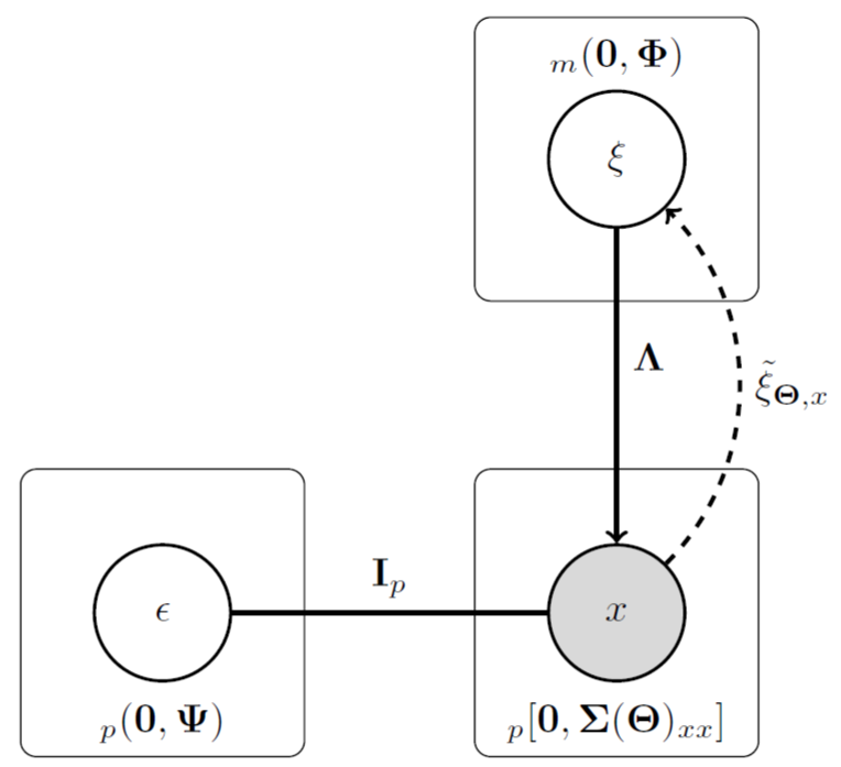
Package purpose

The purpose of the model can be explained with the help of the figure below. It contains a schematic of the factor model we are considering. Nodes indicates random variables and the plates contain postulated distributions (we are assuming specific locations and scales, not distributional shapes). Under this model the correlation matrix of the observables is structured: \mathbf{\Sigma} = \mathbf{\Lambda} \mathbf{\Phi}\mathbf{\Lambda}^{\top} + \mathbf{\Psi}. We thus have a top-down generative model with \xi the latent causal source for the observable x.

The purpose of the package is to:

• Learn (estimate) the weight parameters associated with the model.

• Retrieve the causal latent source through the learned parameters and the marginal behavior of x. In the Machine Learning and AI communities this is understood as finding the latent representation. In the Psychometrics and Statistics communities this is understood as factor scoring.

• Perform uncertainty quantification regarding the retrieved latent source data.

Given the above described generality of the model, the package also aims to bridge the Statistics, Psychometrics, and AI communities. As is described in the function details below, to function in line with its purpose the data only needs to adhere to p > n - 1 > m. In fact, the package is very suited for p \gg n - 1 > m data.

Future

For future updates we will be considering, amongst others, extensions to tensor data (including, for example, a time dimension) and amenities for image compression.

Author(s)

Maintainer: Carel F.W. Peeters carel.peeters@wur.nl (ORCID) [copyright holder]

R data object with metabolomics data on patients with Alzheimer's Disease

Description

ADMdata contains 1 object related to metabolomics data on patients with Alzheimer's Disease (AD).

Details

ADmbolites is a matrix containing metabolic expressions of 230 metabolites (columns) on 87 samples (rows). The data pertain to patients with a known genetic predisposition for AD.

See description.

Author(s)

Carel F.W. Peeters carel.peeters@wur.nl

Source

de Leeuw, F., Peeters, C.F.W., Kester, M.I., Harms, A.C., Struys, E., Hankemeijer, T., van Vlijmen, H.W.T., van Duijn, C.M., Scheltens, P., Demirkan, A., van de Wiel, M.A., van der Flier, W.M., and Teunissen, C.E. (2017). Blood-based metabolic signatures in Alzheimer's Disease. Alzheimer's & Dementia: Diagnosis, Assessment & Disease Monitoring, 8: 196-207.

Examples

data(ADMdata)

## Look at head of data matrix
head(ADmbolites)

Factor analytic metrics for (in)determinacy evaluation

Description

Function that produces metrics on the (degree of) determinacy (uncertainty) of the retrieved latent representation.

Usage

HAMMER.determinacy(H)

Arguments

Details

When one has obtained a factor solution and obtained the factor scores (i.e., obtained the factor analytic data representation) it is of interest to evaluate the uncertainty surrounding the latent representation. In the Psychometric community this topic is known as (the evaluation of) factor indeterminacy and it is closely related to the topic of latent variable collapse in the variational autoencoder framework for deep generative modeling (Peeters, 2026).

The function produces several individual (i.e., per latent factor) and global (i.e., over the collection of latent factors) metrics. The following individual metrics are evaluated with the sample estimates stemming from a call to HAMMER.estimate:

• The squared multiple correlation coefficient between the best linear predictor (proxy) of the latent factor (see HAMMER.score) and the true latent factor:

  \Big[\mathbf{\Phi} - \big(\mathbf{\Phi}^{-1} - \mathbf{\Lambda}^{\top} \mathbf{\Psi}^{-1}\mathbf{\Lambda}\big)^{-1}\Big]_{kk} \equiv \rho(\hat{\xi}_k,\xi_k)^{2},

  for k = 1,\ldots, m latent factors. One would like these correlations to be close to 1. A coefficient indistinguishable from 1 implies full determinacy.

• The Guttman criterion (Guttman, 1955):

  2\rho(\hat{\xi}_k,\xi_k)^{2} - 1,

  for k = 1,\ldots, m latent factors. It represents the degree of conical contraction of possible directions of the true latent vector around the vector that represents the best linear predictor. The closer to 1, the more determinate the retrieval of the latent data through the linear proxy.

The following global metrics are evaluated with the sample estimates stemming from a call to HAMMER.estimate:

• The mean squared error between the best linear predictor (vector) and the true latent vector:

  \|\xi - \hat{\xi}\|_{2}^{2} = \mathrm{tr}\big(\mathbf{\Phi}^{-1} - \mathbf{\Lambda}^{\top} \mathbf{\Psi}^{-1}\mathbf{\Lambda}\big)^{-1}.

  The closer to zero the more the collection of retrieved individual factors is determinate.

• The matrix norm of the conditional covariance of \xi|x:

  \Big\|\big(\mathbf{\Phi}^{-1} - \mathbf{\Lambda}^{\top} \mathbf{\Psi}^{-1}\mathbf{\Lambda}\big)^{-1}\Big\|,

  where the norm can be any induced norm as they are equal when p is finite. The closer to zero the more the collection of retrieved individual factors is determinate.

If the number of features p adhering to the model grows, determinacy will increase. Full determinacy is then obtained in the feature-limit. Full details of these topics and other metrics can be found in Peeters (2026).

Value

The function returns a list object:

Author(s)

Carel F.W. Peeters carel.peeters@wur.nl

References

Guttman, L. (1955). The determinacy of factor score matrices with implications for five other basic problems of common factor theory. British Journal of Mathematical and Statistical Psychology, 8: 65–81

Peeters, C.F.W. (2026). Perspectives on latent factor indeterminacy and its implications for data representation.

See Also

HAMMER.dimension, HAMMER.estimate, HAMMER.score

Examples

## Obtain some high-dimensional data
## In this case the packaged example data
data(ADMdata)
X = scale(ADmbolites)

## Select dimension
fdim <- HAMMER.dimension(X, maxdim = 20, method = "MP")

## Run estimation algorithm with selected dimension
FA <- HAMMER.estimate(X, m = fdim)

## Obtain the scores/latent representation
scores <- HAMMER.score(FA)

## Asses determinacy latent representation
dmncy <- HAMMER.determinacy(FA)
dmncy$Imetrics
dmncy$Gmetrics

Selection of the latent dimension

Description

Function for estimating the number of latent factors in high-dimensional data.

Usage

HAMMER.dimension(X, maxdim, method = "MP", verbose = TRUE)

Arguments

Details

Under our model the first m eigenvalues will grow without bound while the trailing p - m eigenvalues remain bounded as the number of features grows. Let \mathbf{\Sigma} denote a generic second-moment matrix (correlation matrix or any scaling thereoff, such as the covariance matrix). More specifically then, from the population perspective

\mathbf{\Psi}^{-1/2}\mathbf{\Sigma}\mathbf{\Psi}^{-1/2},

has m eigenvalues equaling \infty and p - m eigenvalues equaling 1 as the number of features grows to infinity. One wants to exploit this eigenconcentration to select the number of latent factors m in an empirical setting. As one will not know \mathbf{\Psi} and as the latent dimension is needed for its estimation, one usually uses a very conservative a priori estimate. A conservative estimate can be based on the assumption that all variance is error variance (a sort of null model): \hat{\mathbf{\Psi}} = \mathrm{diag}\big[\mathtt{var}(\mathbf{X})\big], where \mathtt{var} represents the computational operation retrieving the vector of column variances of the input matrix and where \mathbf{X} is our (mean-centered) data matrix of interest. This approach is scale-equivariant in the sense that it leads to assessing the empirical eigenconcentration of the sample correlation matrix.

It is well-known that sample eigenvalues are distorted. Nevertheless, when the model holds and the number of features is high, eigenconcentration can be observed. We then provide several methods for eigenvalue thresholding of \hat{\mathbf{\Psi}}^{-1/2}\hat{\mathbf{\Sigma}} \hat{\mathbf{\Psi}}^{-1/2}:

• Thresholding using the Marchenko-Pastur law (method = "MP"). The eigenvalues of an iso-tropic covariance matrix stemming from n observations of p-dimensional centered variables follow the Marchenko-Pastur probability density function. This distribution is strictly supported on the interval [\sigma^2(1 - \sqrt{p/n})^2, \sigma^2(1 + \sqrt{p/n})^2] (Marchenko and Pastur, 1967). When p > n this spectrum includes a point-mass at zero. This model is, in a sense, a null-model. Representing a factor model that carries no common variance (signal) and consists solely of (isotropic) error variance (noise). The decision rule is then to consider any eigenvalue that exceeds \sigma^2(1 + \sqrt{p/n})^2 to represent signal and all eigenvalues below \sigma^2(1 + \sqrt{p/n})^2 to represent noise. We use the average variance of the variables as the estimate \hat{\sigma}^2 of \sigma^2. When the data are scaled by \hat{\mathbf{\Psi}}^{-1/2} = \mathrm{diag}\big[\mathtt{var}(\mathbf{X})^{\odot(-1/2)}\big] this naturally defers to 1. The (theoretical) justification of this procedure comes from the Baik–Ben Arous–Péché phase transition (Baik, Ben Arous, and Péché, 2005) in which sufficiently strong factors tend to have sample eigenvalues that separate from the bulk of weak factors that remain buried inside the noise spectrum. Let e_{j'} be the j'th eigenvalue of \hat{\mathbf{\Psi}}^{-1/2}\hat{\mathbf{\Sigma}} \hat{\mathbf{\Psi}}^{-1/2} stemming from the centered and scaled matrix \mathbf{X}\hat{\mathbf{\Psi}}^{-1/2} \in \mathbb{R}^{n \times p}, with j' = 1, \ldots, maxdim. The choice \tilde{m} of m is then made as:

  \tilde{m} = \mathrm{card}\Big\{j' ~|~ e_{j'} > \hat{\sigma}^2\big(1 + \sqrt{p/n}\big)^2\Big\}.

• Thresholding using the eigen ratio (method = "eigenratio"). Extending the reasoning regarding eigenconcentration due to an underlying factor model one expects the following: ratios of consecutive noise-eigenvalues are close to one, ratios of consecutive signal-eigenvalues are moderate, but a transition-ratio (of a signal-eigenvalue over a noise-eigenvalue) will be large. This reasoning was used by Ahn and Horenstein (2013) to propose choosing \tilde{m} of m as:

  \tilde{m} = \arg\max_{j'} \frac{e_{j'}}{e_{j'+ 1}},

  with again j' = 1,\ldots, maxdim.

• Thresholding using a growth ratio (method = "growthratio"). We can extend the reasoning above to collapse in the sequence of eigengaps. At the transition of signal to noise the corresponding eigengap will be large relative to succeeding eigengaps. One would then choose \tilde{m} of m as:

  \tilde{m} = \arg\max_{j'} \frac{e_{j'} - e_{j' + 1}} {e_{j'+ 1} - e_{j'+ 2}},

  with again j' = 1,\ldots, maxdim.

• Thresholding using the mean eigenvalue (method = "meansignal"). In some applications one could desire to retain more factors (to maximize, for example, the retained variance in the latent projection). A simple method would then be to retain those dimensions whose eigenvalue exceeds the mean eigenvalue. Under our scaling, the mean eigenvalue is 1 and the method then concurs with the classic Guttman-Kaiser rule from the Psychometric literature (Kaiser, 1970).

Note that the implementation is efficient due to using the implicitly restarted Lanczos bidiagonalization method (Baglama and Reichel, 2005) on a scaled version of the input matrix X to obtain (through the right-singular pairs) the top maxdim eigenpairs of \hat{\mathbf{\Psi}}^{-1/2}\hat{\mathbf{\Sigma}}\hat{\mathbf{\Psi}}^{-1/2}. Operating on (scalings of) X instead of directly on \hat{\mathbf{\Psi}}^{-1/2}\hat{\mathbf{\Sigma}}\hat{\mathbf{\Psi}}^{-1/2} lowers the computational complexity from quadratic in p to linear in p and avoids direct computation and storage of \hat{\mathbf{\Sigma}}.

Value

The function returns an integer indicating the estimated dimension under the chosen method. When verbose = TRUE additional information is printed on-screen.

Note

Note that the input argument X is assumed to be centered. The data matrix may also be scaled. Hence, at least center the data matrix before feeding it to the function.

The intrinsic latent dimension of the standardized data equals, under the model considered, the intrinsic latent dimension of any scaling of that data.

The retained factors should all have eigenvalues exceeding 1. This condition is trivially satisfied for the implemented metrics when the model approximately holds and the number of features grows very large.

If the function returns an integer equal to argument maxdim one has possibly set said argument too low. It is then wise to increase this argument and rerun the procedure.

Author(s)

Carel F.W. Peeters carel.peeters@wur.nl

References

Baglama, J. and Reichel, L. (2005). Augmented implicitly restarted Lanczos bidiagonalization methods. SIAM Journal on Scientific Computing, 27: 19–42.

Baik, J, Ben Arous, B, and Péché, S. (2005). Phase transition of the largest eigenvalue for nonnull complex sample covariance matrices. Annals of Probability, 33: 1643–1697.

Kaiser, H.F. (1970). A second-generation little jiffy. Psychometrika, 35: 401–415.

Marchenko, V.A. and Pastur, L.A. (1967) The distribution of eigenvalues in certain sets of random matrices. Matematicheskii Sbornik, 72: 507–536.

Peeters, C.F.W. (2026). Perspectives on latent factor indeterminacy and its implications for data representation.

See Also

HAMMER.estimate

Examples

## Obtain some high-dimensional data
## In this case the packaged example data
data(ADMdata)
X = scale(ADmbolites)

## Select dimension
HAMMER.dimension(X, maxdim = 20, method = "MP")

Factor analytic parameter learning for high-dimensional data

Description

Function that performs high-dimensional factor analytic parameter learning. That is, it estimates the parameter matrices of the generic factor model given in the package description above.

Usage

HAMMER.estimate(X, m, pinit = 0.1, ccrit = 1e-04, rotation = "none")

Arguments

Details

The function is based on a fixed-point iteration algorithm build around a set of canonical estimating equations. The canonical estimating equations represent the factor model in the canonical orthogonal reflection. The computational complexity of the procedure is linear in the number of features/variables. It achieves this low complexity by using the implicitly restarted Lanczos bidiagonalization method on a scaled version of the input matrix X to obtain (through the right-singular pairs) the top m eigenpairs of the focal error-variance whitened covariance matrix. The procedure then delivers a very swift implementation of canonical factor analysis suited for p > n data. In fact, the procedure is very suited for situations in which p \gg n - 1 > m. The procedure is scale-equivariant, implying that the estimates resulting from the standardized data differ from the estimates resulting from a scaling of the standardized data only by the scaling factors. The procedure is also distribution-free.

Simple structure rotations can be employed to enhance the interpretability of the loadings (and thus the latent factors). Simple structure rotations are geared towards approximately sparse solutions. If rotation = "orthogonal", the Varimax criterion (Kaiser, 1958) for orthogonal simple structure rotation is employed. If rotation = "oblique", the Promax criterion (Hendrickson and White, 1964) for oblique simple structure is employed. The default is no rotation, giving the canonical parameter solution.

Further details can be found in Peeters (2026), especially Section 3.3.

Value

The function returns a list object of the HAMMER class:

Note

Note that the input argument X is assumed to be centered. The data matrix may also be scaled. Hence, at least center the data matrix before feeding it to the function.

Also note that the orthogonal Varimax rotation criterion is implemented with normalization. Hence, it is scale-equivariant. That means that running the algorithm with no rotation or with orthogonal rotation implies scale-equivariance. The oblique Promax rotation criterion is not scale-equivariant. Hence, using the oblique rotation implies that the obliquely rotated loadings are not scale-equivariant.

The dimension m of the latent factor can be determined with the help of the HAMMER.dimension function.

Author(s)

Carel F.W. Peeters carel.peeters@wur.nl

References

Hendrickson, A. E. and White, P. O. (1964). PROMAX: A quick method for rotation to oblique simple structure. British Journal of Mathematical & Statistical Psychology, 17: 65–70.

Kaiser, H. F. (1958). The Varimax criterion for analytic rotation in factor analysis. Psychometrika, 23: 187–200.

Peeters, C.F.W. (2026). Perspectives on latent factor indeterminacy and its implications for data representation.

See Also

HAMMER.dimension, HAMMER.score

Examples

## Obtain some high-dimensional data
## In this case the packaged example data
data(ADMdata)
X = scale(ADmbolites)

## Select dimension
fdim <- HAMMER.dimension(X, maxdim = 20, method = "MP")

## Run estimation algorithm with selected dimension
HAMMER.estimate(X, m = fdim)

Factor analytic representation learning for high-dimensional data

Description

Function that finds, given a factor solution, the low-dimensional generative source data. In the learning community this is understood as 'finding the representation'. In the Psychometrics community this is understood as 'factor scoring'.

Usage

HAMMER.score(H)

Arguments

Details

Once a factor model is fitted (the parameters are learned) one may desire an estimate of the score each sample/object/individual would obtain on each of the latent factors. Such scores are referred to as factor scores. These scores represent the retrieval of the generative latent source data. From another perspective, they provide a representation of the high-dimensional data in low-dimensional latent space. The function swiftly, given an output object stemming from the HAMMER.estimate function, produces Thomson-type scores (Thomson, 1939). These may be viewed as (empirical) Bayesian-type scores and can also be justified as the best linear predictor of the latents given the observables. Out of all linear predictors, this one has the lowest mean-squared error between the predictor (proxy of the latent variable) and the latent variable. Moreover, when the factor model holds, this linear predictors retrieves the true latent factor \xi, irrespective of the distribution of x. These and further details can be found in Peeters (2026).

Value

The function returns a data.frame containing the factor scores. Observations are represented in the rows. Each column represents a latent factor.

Note

The factor scores obtained through the best linear predictor are scale-invariant. The determinacy of the retrieved latent factors can be assessed with the HAMMER.determinacy function.

Author(s)

Carel F.W. Peeters carel.peeters@wur.nl

References

Peeters, C.F.W. (2026). Perspectives on latent factor indeterminacy and its implications for data representation.

Thomson, G. (1939). The Factorial Analysis of Human Ability. London: University of Londen Press.

See Also

HAMMER.dimension, HAMMER.estimate, HAMMER.determinacy

Examples

## Obtain some high-dimensional data
## In this case the packaged example data
data(ADMdata)
X = scale(ADmbolites)

## Select dimension
fdim <- HAMMER.dimension(X, maxdim = 20, method = "MP")

## Run estimation algorithm with selected dimension
FA <- HAMMER.estimate(X, m = fdim)

## Obtain the scores/latent representation
HAMMER.score(FA)