
Felipe MENDEZ and Benjamin RENARD (INRAE) February 2026
ShiftHappens is an R package for detecting,
visualizing and estimating shifts, with a specific focus on hydrology
and hydrometry applications. The package is derived from previous works,
in particular:
You can install the latest stable version from CRAN [recommended] with:
install.packages('ShiftHappens')or the development version from Github [may be unstable] with:
devtools::install_github('benRenard/ShiftHappens')The package can then be loaded with:
library(ShiftHappens)The most common segmentation task is to look for changes in a time series.
The dataset RhoneRiverAMAX coming with the package
contains annual maximum stages (H, \(m\)) and discharges (Q, \(m^3.s^{-1}\)) for the Rhône River at
Beaucaire, France, along with the associated uncertainties expressed as
standard deviations (uH and uQ). A shift is
visually apparent in the stage series around 1970. For more details on
this dataset, see Lucas et
al. (2023).
plot(RhoneRiverAMAX$Date,RhoneRiverAMAX$H)
To segment a series of observations without knowing the number of
segments, we recommend starting with the function
Segmentation_Recursive. With its default arguments, this
function attempts to split the series into two segments using the method
described in Gombay and Horvath (1994), then if successful tries to
further split each obtained segment into two sub-segments, and so on
until all segments cannot be further split. The function returns an
object (see ?recursiveSegmentation) that can be plotted
(see ?plot.recursiveSegmentation).
sg=Segmentation_Recursive(time=RhoneRiverAMAX$Date,
                         obs=RhoneRiverAMAX$H,
                         u=RhoneRiverAMAX$uH)
sg$shifts # estimated shifts
#>          tau  I95_lower  I95_upper id_iteration
#> 1 1967-03-10 1967-04-19 1971-02-28            1
plot(sg)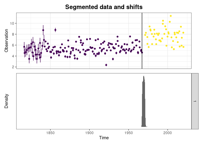
For an illustration with more detected segments, consider segmenting
the series of discharge uncertainties uQ: the many detected
changes reflect changes in the measurement process along the years.
sg=Segmentation_Recursive(time=RhoneRiverAMAX$Date,
                          obs=RhoneRiverAMAX$uQ)
sg$shifts
#>          tau  I95_lower  I95_upper id_iteration
#> 1 1841-10-27 1841-11-05 1842-09-15            1
#> 5 1855-10-21 1846-01-06 1856-05-22            6
#> 3 1858-03-04 1856-07-29 1939-11-06            4
#> 8 1889-01-01 1879-12-23 1920-01-28           12
#> 6 1934-05-01 1932-08-14 1935-10-22            7
#> 2 1952-12-01 1952-01-23 1956-02-08            3
#> 7 1967-03-10 1966-07-16 1971-02-15            8
#> 4 1975-09-16 1974-08-13 1982-10-27            5
plot(sg)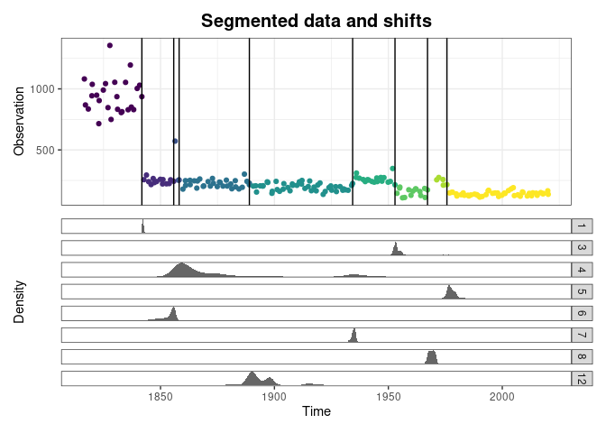
It is also possible to visualize the recursion tree:
plot(sg$tree)
If the number of segments is known, the function
Segmentation_Engine can be used. It returns an object (see
?simpleSegmentation) that can be plotted. Note that if the
desired number of segments is larger than two, the aforementioned method
of Gombay and Horvath (1994) is replaced by the bayesian method
described by M. Darienzo et al. (2021). The package RBaM needs to be installed
in this case.
sg=Segmentation_Engine(time=RhoneRiverAMAX$Date,
                       obs=RhoneRiverAMAX$uQ,
                       nS=4)
plot(sg)
When the number of segments is unknown, the function
Segmentation will try all possible numbers up to
nSmax, and automatically select the most appropriate.
sg=Segmentation(time=RhoneRiverAMAX$Date,
                obs=RhoneRiverAMAX$H,
                nSmax=4)
plot(sg)
In some cases, the objective is not to assess whether the properties of a variable \(x\) has changed, but rather to assess whether the relation between two variables \(x\) and \(y\) has changed. A possible approach for doing so is to model the relation between \(x\) and \(y\) and to look for changes in the residuals of the model (i.e. observed values of \(y\) minus predicted values).
The dataset ArdecheRiverGaugings coming with the package
contains joint measurements of stage (H, \(m\)) and discharge (Q, \(m^3.s^{-1}\)) for the Ardèche River at
Meyras station, France, along with the associated discharge
uncertainties expressed as standard deviations (uQ). The
figure suggests the existence of at least two distinct relations. For
more details on this dataset, see Mansanarez et al. (2019).
plot(ArdecheRiverGaugings$H,ArdecheRiverGaugings$Q)
The function Segmentation_RecursiveModeling fits a model
between \(x\) and \(y\) and then segment the residuals. If
several segments are detected, the model is fitted again on each
obtained segment and the segmentation is re-applied, and so on until all
segments cannot be further split. By default the model used is a simple
linear regression between \(x\) and
\(y\). The function returns an object
(see ?recursiveModeling) that can be plotted (see
?plot.recursiveModeling).
sg=Segmentation_RecursiveModeling(x=ArdecheRiverGaugings$H,
                                  y=ArdecheRiverGaugings$Q,
                                  uY=ArdecheRiverGaugings$uQ,
                                  time=ArdecheRiverGaugings$Date)
plot(sg)
It is possible to replace the upper panel showing the relation between \(x\) and \(y\) by a time series of \(y\) (or \(x\)).
plot(sg,dataPlotType='ty')
The linear regression model illustrated previously is not a very good
model for the relation between stage \(H\) and discharge \(Q\). A rating curve model such as
the one described by Le Coz et al. (2014) is a much better choice. The
function Segmentation_RecursiveModeling has an argument
Fit_funk that allows passing a function fitting any other
model. Here the BaRatin
model, specifically designed for rating curves, is used. A detailed
description of the BaRatin method can be found here, with
a specific explanation on how to use BaRatin in R being
given here.
# Define control matrix: columns are controls, rows are stage ranges.
# See https://baratin-tools.github.io/en/doc/topics/hydraulic-analysis/
controlMatrix=rbind(c(1,0,0),c(0,1,0),c(0,1,1))
# Define parameters of the model
k1=RBaM::parameter(name='k1',init=-0.6,prior.dist='Gaussian',prior.par=c(-0.6,0.5))
a1=RBaM::parameter(name='a1',init=exp(2.65),prior.dist='LogNormal',prior.par=c(2.65,0.35))
c1=RBaM::parameter(name='c1',init=1.5,prior.dist='Gaussian',prior.par=c(1.5,0.025))
k2=RBaM::parameter(name='k2',init=0,prior.dist='Gaussian',prior.par=c(0,1))
a2=RBaM::parameter(name='a2',init=exp(3.28),prior.dist='LogNormal',prior.par=c(3.28,0.33))
c2=RBaM::parameter(name='c2',init=1.67,prior.dist='Gaussian',prior.par=c(1.67,0.025))
k3=RBaM::parameter(name='k3',init=1.2,prior.dist='Gaussian',prior.par=c(1.2,0.2))
a3=RBaM::parameter(name='a3',init=exp(3.46),prior.dist='LogNormal',prior.par=c(3.46,0.38))
c3=RBaM::parameter(name='c3',init=1.67,prior.dist='Gaussian',prior.par=c(1.67,0.025))
priors=list(k1,a1,c1,k2,a2,c2,k3,a3,c3)
# Note: possible to use wrapper function ?Segmentation_BaRatin instead of the function below
sg=Segmentation_RecursiveModeling(x=ArdecheRiverGaugings$H,
                                  y=ArdecheRiverGaugings$Q,
                                  uY=ArdecheRiverGaugings$uQ,
                                  time=ArdecheRiverGaugings$Date,
                                  Fit_funk=Fit_BaRatin,
                                  controlMatrix=controlMatrix,priors=priors)
plot(sg)
Note that each individual plot created by the package is a ggplot that can be customized. For instance:
plot(sg,type='data')+ggplot2::labs(x='Stage',y='Discharge')+
  ggplot2::scale_y_continuous(trans='log')
This method is specific to the hydrometry context, and aims at detecting shifts using the stage record, measured at any hydrometric station. The basic idea is that the water level tends to the riverbed level at very low flows. It should therefore be possible to detect changes by looking at the lowest water levels reached during long recession periods.
The dataset ArdecheRiverStage coming with the package
contains the stage time series (H, \(m\)) for the Ardèche River at Meyras
station, France. There seems to be a downward shift around 2008 in the
lowest stage values. For more details on this dataset, see Matteo Darienzo
(2021).
plot(ArdecheRiverStage$Date,ArdecheRiverStage$H,type='l')
The first step is to extract recession events using the function
Extract_Recessions. Many options are available to customize
the definition of recession events, see
?Extract_Recessions. The function returns an object (see
?extractedRecessions) that can be plotted in various ways
(see ?plot.extractedRecessions). Here for instance the
extracted recession events are shown as a function of the calendar date
(left) or the within-recession time (i.e. starting at the beginning of
the recession, right).
rec=Extract_Recessions(time=ArdecheRiverStage$Date,H=ArdecheRiverStage$H,dMin=30)
patchwork::wrap_plots(plot(rec),plot(rec,type='th'))
The next step is to apply a segmentation procedure to a well-chosen
property of the extracted recession events. The simplest way to start is
to get the lowest value of each recession (using utility function
getRecessionMin) and to segment them.
lows=getRecessionMin(rec)
sg=Segmentation_Recursive(obs=lows$H,time=lows$date)
plot(sg)
A more advanced approach is to model the extracted recessions and to
segment the parameter of this model that controls the asymptotic low
stage. Details on this procedure can be found in Matteo Darienzo
(2021) (Chapter 3). First, the function Fit_Recessions
can be used to fit the recession model.
# View available recession models.
# Note that in all equations, the asymptotic stage (when t tends to infinity)
# is equal to parameter beta_k
getRecessionEquations()
#> $M1
#> [1] "alpha_k*exp(-lambda*t)+beta_k"
#>
#> $M2
#> [1] "alpha1_k*exp(-lambda1*t)+alpha2*exp(-lambda2*t)+beta_k"
#>
#> $M3
#> [1] "alpha1_k*exp(-lambda1*t)+alpha2_k*exp(-lambda2*t)+beta_k"
#>
#> $M4
#> [1] "alpha1_k*exp(-lambda1*t)+alpha2*exp(-lambda2*t)+alpha3*exp(-lambda3*t)+beta_k"
#>
#> $M5
#> [1] "alpha1_k*exp(-lambda1*t)+alpha2_k*exp(-lambda2*t)+alpha3*exp(-lambda3*t)+beta_k"
#>
#> $M6
#> [1] "alpha_k*exp(-lambda*t^eta)+beta_k"
#>
#> $M7
#> [1] "alpha_k*exp(-lambda_k*t^eta)+beta_k"
#>
#> $M8
#> [1] "alpha_k/((1+lambda*t)^eta)+beta_k"
#>
#> $M9
#> [1] "alpha_k/((1+lambda_k*t)^eta)+beta_k"
# Fit one of the models
f=Fit_Recessions(rec,equation='M7',
                 # The line below aims at speeding up computations,
                 # but it is advised to make definitive runs
                 # with the default MCMC options
                 mcmc_options=RBaM::mcmcOptions(nAdapt=25,nCycles=20))
patchwork::wrap_plots(plot(f),plot(f,type='ty'),ncol=1)
Second, the parameters controlling the recession asymptotic stages
can be extracted and segmented. Note that the wrapper function
Segmentation_Recessions can be used to perform the whole
model-then-segment analysis in one go.
betas=f$parameters[1:max(rec$index),]
sg=Segmentation_Recursive(obs=betas$value,u=betas$u)
plot(sg)