Package {VsusP}

Title:	Variable Selection Using Shrinkage Priors
Version:	1.1.0
Description:	Select variables from shrinkage-prior posterior coefficient draws using sequential two-means clustering from Li and Pati (2017) <doi:10.1016/j.csda.2016.10.008>. Estimate a signal count at each tuning threshold and rank coefficients by posterior median absolute magnitude. Accept supplied coefficient draws or fit Gaussian shrinkage regression through 'bayesreg' or native ridge, horseshoe and spike-and-slab samplers. Retain chain identities for diagnostics, prediction and posterior plots. Also provide the signal adaptive variable selector of Ray and Bhattacharya (2018) <doi:10.48550/arXiv.1810.09004>, decoupled shrinkage and selection with the adaptive-L1 approximation of Hahn and Carvalho (2015) <doi:10.1080/01621459.2014.993077>, optional exact two-cluster fitting, basic two-means selection, exact-zero spike-and-slab inclusion summaries and tuning sensitivity summaries.
License:	GPL (≥ 3)
Encoding:	UTF-8
RoxygenNote:	7.3.3
Imports:	bayesreg, graphics, stats, utils
Suggests:	posterior (≥ 1.6.0), covr, MASS, knitr, rmarkdown, tinytex, testthat (≥ 3.2.0)
Config/testthat/edition:	3
Maintainer:	Nilson Chapagain <nilson.chapagain@gmail.com>
URL:	https://github.com/nilson01/VsusP-variable-selection-using-shrinkage-priors
BugReports:	https://github.com/nilson01/VsusP-variable-selection-using-shrinkage-priors/issues
VignetteBuilder:	knitr
NeedsCompilation:	no
Packaged:	2026-10-28 15:34:37 UTC; nilson
Author:	Nilson Chapagain [aut, cre], Debdeep Pati [aut]
Repository:	CRAN
Date/Publication:	2026-10-28 17:00:02 UTC

Variable selection from Bayesian shrinkage priors

Description

Select variables from posterior coefficient draws, or fit Gaussian shrinkage regression and summarize its posterior. Selection and posterior fitting are separate operations.

Gaussian regression

FitRidge(), FitHorseshoe() and FitSpikeSlab() retain separate iteration, chain and predictor axes. PosteriorDraws() pools chains for selection. Use summary and predict for posterior estimates and pointwise intervals. ChainDiagnostics(), PlotTrace() and PlotAutocorrelation() keep chain identities. Successful sampling alone does not establish convergence.

Selection

Sequential2MeansBeta() and TwoMeansBeta() summarize supplied draws; S2MSensitivity() compares thresholds. SpikeSlabSelection() counts exact nonzero coefficients. SAVS() and DSS() construct sparse coefficient summaries and can return no selected variables. Clustering counts are not inclusion probabilities or false-discovery guarantees.

Fixed-posterior checks

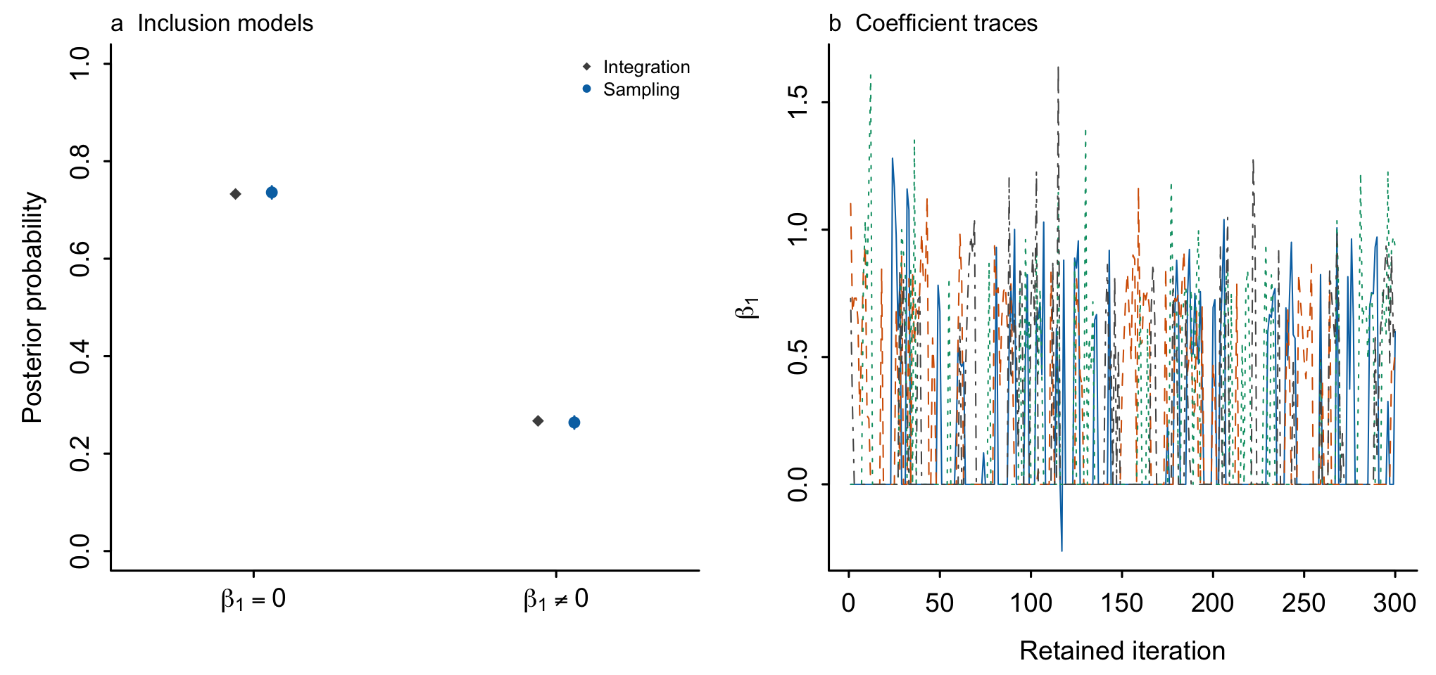
The following plots use five observations and one predictor. Four chains retain 3000 iterations each after 1000 burn-in iterations. HS denotes horseshoe and SS denotes spike-and-slab. Sampled posterior summaries are compared with independent numerical integration. The audit tolerance is the larger of 0.01 and six estimated Monte Carlo standard errors, computed using 100-draw batches. The shaded range is an audit criterion, not a confidence interval. These checks do not establish performance across repeated datasets.

The spike-and-slab model has two possible inclusion states. Points compare their integrated and sampled probabilities; error bars are plus or minus 1.96 estimated Monte Carlo standard errors. Traces display the first 300 retained coefficient draws per chain. All retained draws enter the summaries.

Author(s)

Maintainer: Nilson Chapagain nilson.chapagain@gmail.com (ORCID)

Authors:

• Debdeep Pati debdeep@tamu.edu

References

Li, H. and Pati, D. (2017). Variable selection using shrinkage priors. Computational Statistics & Data Analysis, 107, 107–119. doi:10.1016/j.csda.2016.10.008.

See Also

FitGaussian(), PlotCoefficients(), PlotInclusion(), vignette("VsusPVignette")

Calculate diagnostics with explicit chain identities

Description

Delegate rank R-hat, bulk/tail effective sample size and mean Monte Carlo standard error to the optional posterior package.

Usage

ChainDiagnostics(draws, feature.names = NULL)

Arguments

Details

At least four retained iterations per chain are required. Install posterior separately when using this function. No chain is reconstructed from a pooled draw matrix. R and Python diagnostics can differ slightly between backend versions; both use the cited rank-based definitions.

Value

Data frame with rhat, ess.bulk, ess.tail, mcse.mean and status. A single chain has unavailable R-hat. Constant variables have unavailable diagnostics. Finite diagnostic values do not certify convergence.

References

Vehtari et al. (2021). Rank-normalization, folding, and localization: An improved R-hat for assessing convergence of MCMC. doi:10.1214/20-BA1221.

Examples

if (requireNamespace("posterior",quietly=TRUE)) {
  a <- array(sin(seq_len(800)),c(100,2,4))
  ChainDiagnostics(a)
}

Sparse prediction with the DSS adaptive-lasso approximation

Description

Approximate the posterior-mean linear predictor with a sparse coefficient vector using the decoupled shrinkage and selection (DSS) adaptive-L1 criterion of Hahn and Carvalho (2015), equation (21).

Usage

DSS(X, beta, lambda, tol = 1e-08, max.iter = 10000L)

Arguments

Details

Here beta represents the posterior mean, and X contains the prediction points at which the sparse predictor should approximate X beta. These need not be the observations used to fit the posterior. The objective is

n^{-1}\|X\bar{\beta}-X\gamma\|_2^2 + \lambda\sum_{j:\bar{\beta}_j\ne0}|\gamma_j|/|\bar{\beta}_j|.

This is the paper's adaptive-L1 approximation, not exact minimization of its L0 counting penalty.

For positive lambda, a zero beta entry constrains the corresponding sparse coefficient to zero, the infinite-weight limit. For lambda = 0, beta itself is returned as a least-squares minimizer. No intercept, centering or scaling is added. Exclude the intercept and keep its contribution separately. The adaptive criterion is unchanged by rescaling predictor columns and inversely rescaling beta, apart from floating-point error and nonunique solutions. Changing response units requires changing lambda accordingly.

Cyclic coordinate descent solves the convex surrogate in the transformed design X times abs(beta). The KKT error is divided by the larger of lambda and the largest absolute initial gradient. A result is converged when this ratio is at most tol. The iteration limit produces a warning and converged = FALSE; inspect this flag before using the selection. Overflow and detected underflow in transformed columns, norms, sparse coefficients or squared errors are rejected. With dependent predictor columns, coefficients and selected sets need not be unique; coordinates are visited in the supplied column order.

Squared error here measures approximation to the supplied posterior mean at X, not held-out predictive error. The function does not select lambda, compute inclusion probabilities or establish false-discovery control.

Value

A vsusp_sparse list with coefficients, selected (integer column indices, possibly integer(0)), p, lambda, fitted (X coefficients), mse (mean squared approximation error), penalty (weighted L1 penalty including lambda), objective (mse + penalty), iterations, kkt.error (relative KKT error) and converged. Numerical diagnostics concern the convex surrogate only.

References

Hahn, P. R. and Carvalho, C. M. (2015). Decoupling Shrinkage and Selection in Bayesian Linear Models: A Posterior Summary Perspective. Journal of the American Statistical Association, 110(509), 435-448. doi:10.1080/01621459.2014.993077.

Examples

X <- diag(2)
DSS(X, c(2, .1), lambda = .2)$coefficients
DSS(X, c(2, .1), lambda = 10)$selected

Fit native Gaussian shrinkage regression

Description

Fit ridge, horseshoe or exact-zero spike-and-slab regression while retaining separate iteration and chain axes. Existing bayesreg wrappers are unchanged.

Usage

FitGaussian(
  X,
  y,
  prior = c("ridge", "horseshoe", "spike-slab"),
  draws = 1000L,
  burnin = NULL,
  chains = 4L,
  seed = NULL,
  prior.scale = 1,
  feature.names = colnames(X)
)

FitRidge(
  X,
  y,
  draws = 1000L,
  chains = 4L,
  prior.scale = 1,
  seed = NULL,
  feature.names = colnames(X)
)

FitHorseshoe(
  X,
  y,
  draws = 1000L,
  burnin = 1000L,
  chains = 4L,
  seed = NULL,
  feature.names = colnames(X)
)

FitSpikeSlab(
  X,
  y,
  draws = 1000L,
  burnin = 1000L,
  chains = 4L,
  seed = NULL,
  feature.names = colnames(X)
)

Arguments

Details

The likelihood is Gaussian with a flat intercept prior. Predictors and response are centered, not standardized. The intercept is integrated during coefficient/variance updates and then sampled on the original scale. The residual-variance prior is IG(1.5,1.5), with density proportional to x^(-a-1) exp(-b/x). Ridge coefficients have conditional variance sigma2 * prior.scale^2. Horseshoe local and global scales independently follow half-Cauchy(0,1) priors. For spike-and-slab, inclusion probability follows Beta(1,15), slab variance multipliers follow IG(1.5,1.5), and excluded coefficients are exactly zero. R and Python use different random-number streams. Retained draws do not prove convergence.

Value

A vsusp_fit list with beta (iteration by chain by predictor), intercept and sigma2 (iteration by chain), prior, feature.names, extra scale/inclusion draws and metadata. Draws count retained iterations.

References

Li, H. and Pati, D. (2017). Variable selection using shrinkage priors. Computational Statistics & Data Analysis, 107, 107–119. doi:10.1016/j.csda.2016.10.008.

Makalic, E. and Schmidt, D. F. (2016). A simple sampler for the horseshoe estimator. doi:10.1109/LSP.2015.2503725.

Bhattacharya, A., Chakraborty, A. and Mallick, B. K. (2016). Fast sampling with Gaussian scale-mixture priors in high-dimensional regression. doi:10.1093/biomet/asw042.

See Also

PosteriorDraws(), ChainDiagnostics()

Examples

X <- cbind(x1 = c(-2,-1,0,1,2,0), x2 = c(0,1,-1,0,1,-1))
fit <- FitRidge(X, c(-4,-2,0,2,4,0), draws=100, chains=2, seed=8)
summary(fit)
predict(fit, X[1:2,,drop=FALSE])

Plot the sequential two-means tuning path

Description

Display the estimated signal count at each threshold to support a choice of tuning parameter. The function does not choose a threshold or H.

Usage

OptimalHbi(bi, Hbi)

Arguments

Value

Invisible NULL. A plot is drawn on the current graphics device.

References

Li, H. and Pati, D. (2017). Variable selection using shrinkage priors. Computational Statistics & Data Analysis, 107, 107–119. doi:10.1016/j.csda.2016.10.008.

See Also

Sequential2MeansBeta()

Examples

Beta <- rbind(c(.01, .02, .03, .3, .31, 10, 11),
              c(-.01, -.02, -.03, -.3, -.31, -10, -11))
set.seed(1)
result <- Sequential2MeansBeta(Beta, .1, .5, 2)
OptimalHbi(result$b.i, result$H.b.i)

Plot within-chain sample autocorrelations

Description

Plot within-chain sample autocorrelations

Usage

PlotAutocorrelation(draws, variable = 1L, max.lag = 40L, ...)

Arguments

Value

Invisibly, a lag by chain autocorrelation matrix. Constant chains have NA autocorrelations, rather than evidence of mixing.

Example figure

Within-chain autocorrelations from all 3000 retained horseshoe draws per chain in the same example.

Plot posterior coefficient summaries

Description

Plot posterior coefficient summaries

Usage

PlotCoefficients(object, interval = 0.95, selected = integer(0), ...)

Arguments

Value

Invisibly, the displayed summary data frame. No model is fitted.

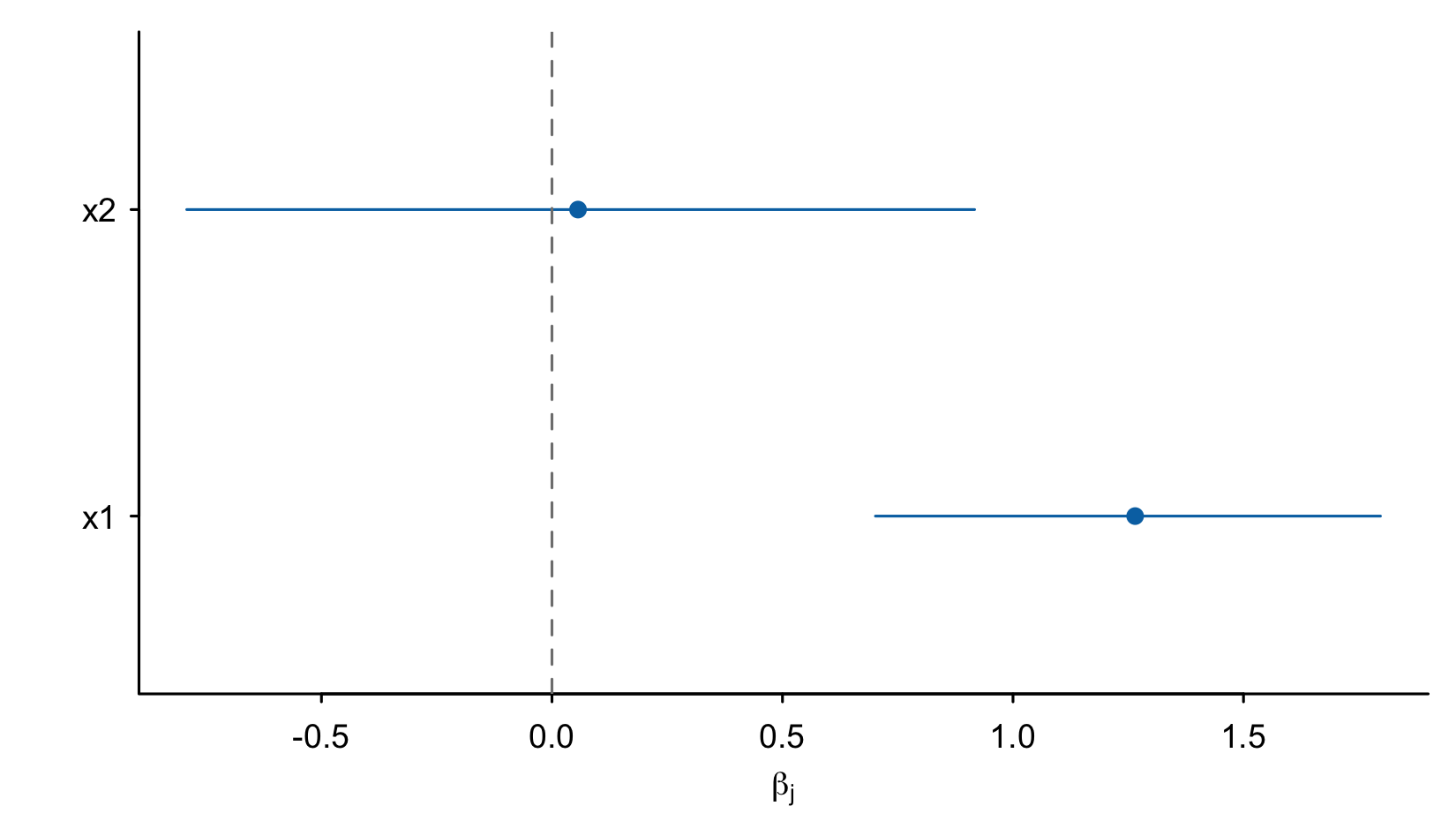
Example figure

Posterior means and 95 percent equal-tail intervals for a six-observation ridge example.

Examples

X <- matrix(c(-1,0,1,2),ncol=1)
fit <- FitRidge(X,c(-1,0,1,2),draws=30,chains=2,seed=1)
PlotCoefficients(fit)

Plot exact spike inclusion frequencies

Description

Plot exact spike inclusion frequencies

Usage

PlotInclusion(object, ...)

Arguments

Value

Invisibly, the displayed frequencies. The dashed line marks the median-probability-model cutoff; it is not an error-control threshold.

Example figure

Inclusion frequencies from four fixed coefficient rows. The dashed line marks 0.5.

Plot chains without pooling their iterations

Description

Plot chains without pooling their iterations

Usage

PlotTrace(draws, variable = 1L, ...)

Arguments

Value

Invisibly, the iteration by chain matrix displayed.

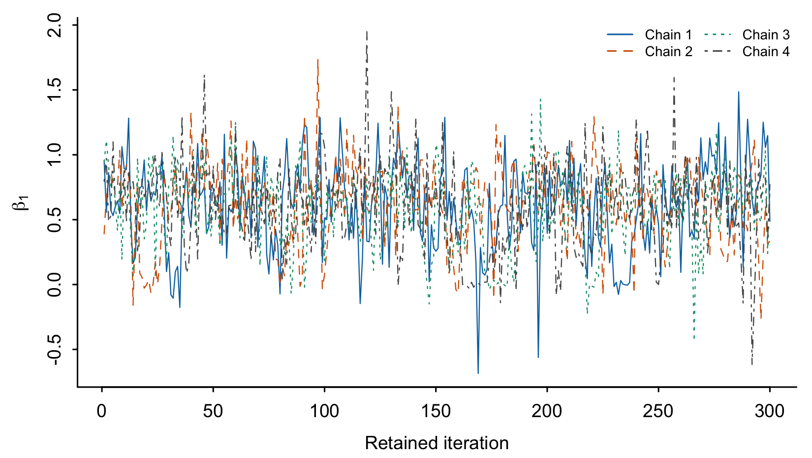
Example figure

First 300 retained draws from each of four horseshoe chains in the five-observation example. This excerpt is not a convergence assessment.

Pool retained coefficient draws for selection

Description

Pool retained coefficient draws for selection

Usage

PosteriorDraws(object)

Arguments

Value

Numeric matrix with draws in rows and predictors in columns. Chains are combined only in this returned matrix; the fit retains its chain axes.

Examples

X <- matrix(c(-1,0,1,2), ncol=1)
fit <- FitRidge(X,c(-1,0,1,2),draws=20,chains=2,seed=3)
dim(PosteriorDraws(fit))

Summarize sensitivity to sequential two-means thresholds

Description

Compare signal counts and selected sets over an explicit threshold grid. This function does not choose a threshold.

Usage

S2MSensitivity(
  Beta,
  b.i,
  clustering = c("kmeans", "exact"),
  small.set = c("legacy", "refine")
)

Arguments

Details

The Jaccard similarity is the intersection size divided by the union size. It describes overlap, not statistical accuracy. Count frequencies are clustering frequencies, not posterior inclusion probabilities. A stable tuning path need not recover the true variable set.

Value

A vsusp_tuning list with b.i, H.b.i and abs.post.median as in Sequential2MeansBeta, plus frequencies (a list of per-draw count tables), selected (a list of selected-index vectors), mode.proportion (the fraction of draws giving the modal count), and jaccard.previous (selected-set overlap with the preceding grid entry; NA for the first entry). The shared p field permits passing this summary to S2MVarSelectionV1.

See Also

Sequential2MeansBeta(), OptimalHbi()

Examples

Beta <- rbind(c(.01,.02,.03,.3,.31,10,11),
              c(-.01,-.02,-.03,-.3,-.31,-10,-11))
result <- S2MSensitivity(Beta,c(.1,.5),clustering="exact")
result$H.b.i
result$jaccard.previous

Select coefficients by posterior median absolute magnitude

Description

Return the indices of the H largest column medians of absolute draws.

Usage

S2MVarSelection(Beta, H = 5)

Arguments

Details

H is supplied by the caller. This function does not estimate H or test statistical significance.

Value

Integer vector of selected column indices in decreasing order of median absolute magnitude. Equal medians favor larger column indices. H = 0 returns integer(0).

References

Li, H. and Pati, D. (2017). Variable selection using shrinkage priors. Computational Statistics & Data Analysis, 107, 107–119. doi:10.1016/j.csda.2016.10.008.

See Also

S2MVarSelectionV1(), Sequential2MeansBeta()

Examples

Beta <- rbind(c(.01, .02, .03, .3, .31, 10, 11),
              c(-.01, -.02, -.03, -.3, -.31, -10, -11))
set.seed(1)
result <- Sequential2MeansBeta(Beta, .1, .5, 2)
S2MVarSelection(Beta, result$H.b.i[2])
S2MVarSelection(Beta, 0)

Select coefficients from an S2M summary

Description

Select the H largest posterior median absolute coefficients from a summary returned by either S2M fitting function.

Usage

S2MVarSelectionV1(S2M, H = 5)

Arguments

Value

Integer vector of selected column indices, ordered by decreasing median absolute magnitude. Equal medians favor larger column indices. H = 0 returns integer(0).

References

Li, H. and Pati, D. (2017). Variable selection using shrinkage priors. Computational Statistics & Data Analysis, 107, 107–119. doi:10.1016/j.csda.2016.10.008.

See Also

S2MVarSelection(), Sequential2MeansBeta()

Examples

Beta <- rbind(c(.01, .02, .03, .3, .31, 10, 11),
              c(-.01, -.02, -.03, -.3, -.31, -10, -11))
set.seed(1)
result <- Sequential2MeansBeta(Beta, .1, .5, 2)
S2MVarSelectionV1(result, result$H.b.i[2])

Select variables with the signal adaptive variable selector

Description

Apply the closed-form signal adaptive variable selector (SAVS) of Ray and Bhattacharya to a coefficient point estimate, such as a posterior mean. The selected set can be empty.

Usage

SAVS(X, beta)

Arguments

Details

A coefficient is retained when its absolute value cubed, multiplied by the squared norm of its predictor column, exceeds one. Equality gives zero. An exactly zero input coefficient gives zero without division. Direct products are used when their factors are representable. Otherwise logarithms avoid overflow; scores indistinguishable from the threshold within floating-point rounding error are set to zero.

No centering or scaling is performed. Use the same design matrix and units that define beta. SAVS depends on units: changing predictor or response scales can change the selected set. Standardize predictors before fitting if selection on a common predictor scale is wanted.

This function applies equation (2) and Algorithm 1 of the cited preprint. It does not solve the full correlated-design penalized optimization problem. It neither computes inclusion probabilities nor guarantees false-discovery control. Its behavior depends on the supplied estimate.

Value

A vsusp_sparse list with coefficients (sparse estimates), selected (integer column indices), p (number of coefficients), and log.score (log decision scores). selected is integer(0) when every coefficient is set to zero.

Selection pilot

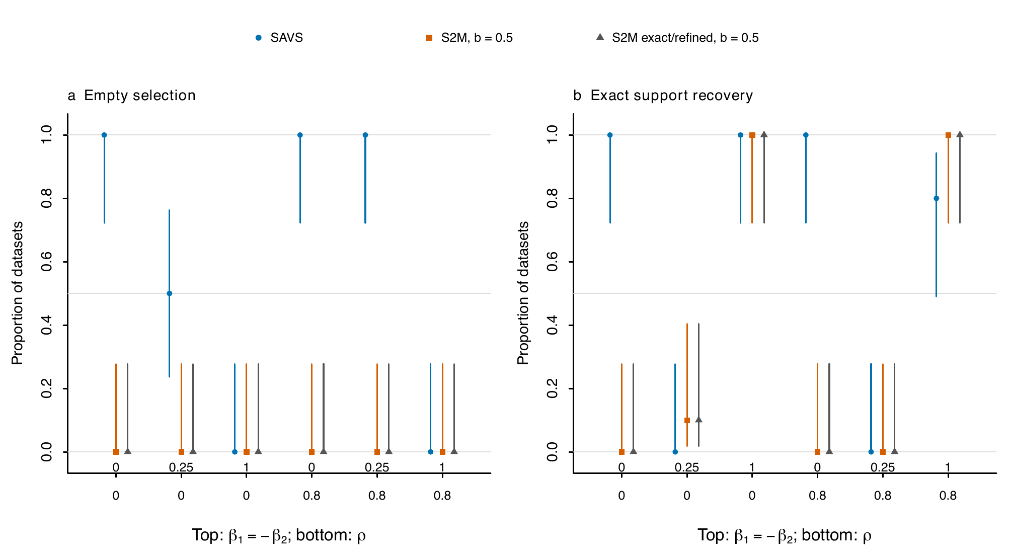
Empty-selection and exact-support proportions in six Gaussian conditions, with ten datasets per condition and 95 percent Wilson intervals. This small pilot does not establish false-discovery control. See the worked guide for the design and interpretation.

References

Ray, P. and Bhattacharya, A. (2018). Signal Adaptive Variable Selector for the Horseshoe Prior. arXiv:1810.09004. https://arxiv.org/abs/1810.09004.

Examples

X <- diag(2)
SAVS(X, c(.1, -.1))$selected
SAVS(X, c(2, 0))$coefficients

Fit Gaussian shrinkage regression and apply sequential two-means

Description

Fit a Gaussian linear model with bayesreg, then apply sequential two-means (S2M) to its coefficient draws. The intercept is excluded from selection.

Usage

Sequential2Means(
  X,
  Y,
  b.i,
  prior = "horseshoe+",
  n.samples = 5000,
  burnin = 2000,
  clustering = c("kmeans", "exact"),
  small.set = c("legacy", "refine")
)

Arguments

Details

All returned draws are used. Thresholds are on the coefficient scale, so predictor scaling affects their interpretation. See Sequential2MeansBeta() for stopping conventions and limitations. A short chain demonstrates the call; assess convergence and effective sample size before using posterior summaries for inference.

Value

A list with Beta (returned draws in rows, predictors in columns), p (number of predictors), b.i (thresholds), H.b.i (modal signal counts), and abs.post.median (column medians of absolute coefficient draws).

References

Li, H. and Pati, D. (2017). Variable selection using shrinkage priors. Computational Statistics & Data Analysis, 107, 107–119. doi:10.1016/j.csda.2016.10.008.

Wang, H. and Song, M. (2011). Ckmeans.1d.dp: Optimal k-means clustering in one dimension by dynamic programming. The R Journal, 3(2), 29–33. doi:10.32614/RJ-2011-015.

See Also

Sequential2MeansBeta(), S2MVarSelectionV1()

Examples

set.seed(12)
X <- matrix(rnorm(120), 40, 3)
Y <- 3 * X[, 1] + rnorm(40)
result <- Sequential2Means(X, Y, c(.1, .5), prior = "ridge",
                           n.samples = 100, burnin = 100)
dim(result$Beta)
S2MVarSelectionV1(result, result$H.b.i[1])

Apply sequential two-means to posterior coefficient draws

Description

Estimate a signal count at each threshold from supplied coefficient draws, following section 2.2.1 of Li and Pati (2017).

Usage

Sequential2MeansBeta(
  Beta,
  lower,
  upper,
  l,
  clustering = c("kmeans", "exact"),
  small.set = c("legacy", "refine"),
  zero.draws = c("error", "empty")
)

Arguments

Details

For each draw, S2M first splits absolute coefficients into two clusters. It saves the lower-mean cluster as the noise candidate set. While the center gap exceeds the threshold, it saves the current lower-mean cluster and splits that set again. At stopping it uses the saved set, rather than the lower cluster from the stopping split.

By default, the implementation retains a candidate set of at most two elements, or a candidate with identical magnitudes, without another split. For an initial pair of distinct magnitudes, the lower singleton is the noise set. An initial draw with identical magnitudes has no lower-mean cluster and is rejected. These are computational boundary conventions. The refine option can change counts when a retained pair has gap greater than b.

H.b.i is the mode of the per-draw signal counts; a frequency tie selects the smaller count. Accepted draws always leave at least one signal, so S2M cannot automatically select an empty model. This clustering summary is not a posterior inclusion probability or an error-control guarantee. Results can depend on kmeans initialization; use set.seed() for reproducibility. The exact backend consumes no random draws. It finds the minimum within-cluster sum of squares in floating-point arithmetic; equal losses choose the earliest sorted cut. Numeric rescaling that collapses distinct values is rejected. An exact clustering optimum does not establish optimal variable selection. Scaling coefficients changes threshold meaning. With zero.draws = "empty", all-zero draws contribute zero to the count frequencies and their row indices are returned as zero.draws. Other constant-magnitude draws remain invalid. This convention does not make S2M an empty-model selector for continuous-prior draws.

Value

A list with p (number of coefficients), b.i (thresholds), H.b.i (modal signal counts), and abs.post.median (column medians of absolute coefficient draws).

References

Li, H. and Pati, D. (2017). Variable selection using shrinkage priors. Computational Statistics & Data Analysis, 107, 107–119. doi:10.1016/j.csda.2016.10.008.

Wang, H. and Song, M. (2011). Ckmeans.1d.dp: Optimal k-means clustering in one dimension by dynamic programming. The R Journal, 3(2), 29–33. doi:10.32614/RJ-2011-015.

See Also

Sequential2Means(), OptimalHbi(), S2MVarSelection()

Examples

Beta <- rbind(c(.01, .02, .03, .3, .31, 10, 11),
              c(-.01, -.02, -.03, -.3, -.31, -10, -11))
set.seed(1)
result <- Sequential2MeansBeta(Beta, .1, .5, 2)
result$H.b.i
S2MVarSelectionV1(result, result$H.b.i[2])

Summarize exact spike-and-slab posterior draws

Description

Estimate inclusion probabilities and return the median probability model (MPM) and the most frequent complete inclusion pattern visited by the draws (the empirical HPPM).

Usage

SpikeSlabSelection(Beta)

Arguments

Details

The MPM includes variables with inclusion frequency greater than or equal to 0.5, as in Li and Pati (2017). The empirical HPPM counts full joint inclusion patterns, rather than combining marginal probabilities. It estimates the highest-probability visited model from the supplied sample; it does not establish the global posterior mode. Model rows are ordered by first occurrence. If model frequencies tie, HPPM uses the first observed tied model; HPPM.ties retains all tied row indices.

Exact zeros are a data contract, not a numerical tolerance. Draws from a continuous shrinkage prior are inappropriate for this summary: small nonzero values count as included. An all-zero draw is the empty model, and an entirely zero matrix returns empty MPM and HPPM selections. This function fits no model and derives no probabilities from clustering.

Value

A vsusp_spike list containing p, inclusion.probability, selected column indices MPM and HPPM, logical matrix visited.models (one distinct model per row), model.frequencies (model row index, draw count, proportion, and first draw), and HPPM.ties (all model row indices tied for largest count).

References

Li, H. and Pati, D. (2017). Variable selection using shrinkage priors. Computational Statistics & Data Analysis, 107, 107–119. doi:10.1016/j.csda.2016.10.008.

Examples

Beta <- rbind(c(1, 0, 0), c(2, 0, 0), c(0, -1, 0), c(0, -2, 0))
SpikeSlabSelection(Beta)

Select variables by the paper's two-means rule

Description

Cluster each draw's absolute coefficients into two groups. The smaller group size estimates the number of signals for that draw. Select the modal number of variables using posterior medians of absolute coefficients.

Usage

TwoMeansBeta(Beta, clustering = c("exact", "kmeans"))

Arguments

Details

This is the 2-M rule in Section 2.1 of Li and Pati (2017). It uses the smaller cluster size, regardless of which cluster has the higher mean. It is distinct from the recursive S2M noise-cluster rule. An equal-size split has that common size. A tied modal count favors the smaller count. Equal posterior medians favor larger column indices, matching S2MVarSelection(). The exact backend favors the earliest cut in sorted magnitudes when objective values tie. The kmeans backend uses R's initialization and RNG; set a seed for reproducibility.

Two-means is undefined for constant magnitudes. As an explicit extension, an all-zero draw has signal count zero and is not clustered. A constant nonzero magnitude draw is rejected before consuming clustering RNG. Neither convention is a published clustering result. H = 0 returns an empty selection. This function summarizes supplied draws; it fits no model. Sparse spike-and-slab draws can give zero medians for every coefficient. Median ties may then select a coefficient never included in any draw. Use SpikeSlabSelection() for summaries based on inclusion frequencies.

Value

A vsusp_selection list containing p, the selected count H, per-draw signal.count, abs.post.median, selected column indices selected, a count table frequencies, the backend clustering, and indices zero.draws of draws handled by the zero-model boundary convention.

References

Li, H. and Pati, D. (2017). Variable selection using shrinkage priors. Computational Statistics & Data Analysis, 107, 107–119. doi:10.1016/j.csda.2016.10.008.

Examples

Beta <- rbind(c(0, .1, 10, 11, 12), c(0, -.1, -10, -11, -12))
TwoMeansBeta(Beta)
TwoMeansBeta(matrix(0, 2, 3))

Posterior coefficient means

Description

Posterior coefficient means

Usage

## S3 method for class 'vsusp_fit'
coef(object, ...)

Arguments

Value

Named numeric vector of posterior coefficient means, excluding the intercept. Intercept draws remain in object$intercept.

Count coefficients in the saved S2M noise set

Description

Count coefficients in the saved S2M noise set

Usage

numNoiseCoeff(Beta.i, b.i_r, clustering = "kmeans", small.set = "legacy")

Arguments

Value

Size of the saved lower-mean candidate set.

Plot a native Gaussian fit

Description

Plot a native Gaussian fit

Usage

## S3 method for class 'vsusp_fit'
plot(x, type = c("coefficients", "trace", "acf", "inclusion"), ...)

Arguments

Value

Invisibly, the displayed numerical values.

Plot a tuning path

Description

Plot a tuning path

Usage

## S3 method for class 'vsusp_tuning'
plot(x, ...)

Arguments

Value

Invisibly, the displayed thresholds and counts, sorted by threshold.

Example figure

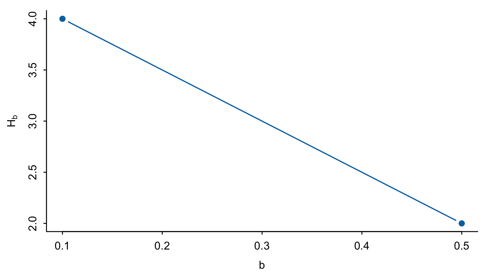
Signal counts at two thresholds for fixed seven-coefficient draws. The path does not select a threshold.

Predict from native Gaussian posterior draws

Description

Predict from native Gaussian posterior draws

Usage

## S3 method for class 'vsusp_fit'
predict(
  object,
  newdata,
  interval = 0.95,
  include.noise = FALSE,
  seed = NULL,
  ...
)

Arguments

Value

List with mean, lower, upper, interval and kind. Intervals are pointwise posterior intervals, not simultaneous bands. kind is "mean" or "observation". Prediction does not refit the model.

Predict using sparse coefficient summaries

Description

Predict using sparse coefficient summaries

Usage

## S3 method for class 'vsusp_sparse'
predict(object, newdata, intercept = 0, ...)

Arguments

Value

Numeric vector. This method returns sparse linear predictions; it supplies no uncertainty interval and does not refit a model.

Summarize native Gaussian posterior draws

Description

Summarize native Gaussian posterior draws

Usage

## S3 method for class 'vsusp_fit'
summary(object, interval = 0.95, ...)

Arguments

Value

Data frame with posterior mean, SD, lower and upper equal-tail limits. SD is NA when only one draw is available.

Summarize basic two-means selection

Description

Summarize basic two-means selection

Usage

## S3 method for class 'vsusp_selection'
summary(object, ...)

Arguments

Value

Named selected indices, preserving the fitted ranking.

Summarize sparse coefficient results

Description

Summarize sparse coefficient results

Usage

## S3 method for class 'vsusp_sparse'
summary(object, ...)

Arguments

Value

Data frame with coefficient values and a selected indicator.

Summarize exact spike-and-slab inclusion draws

Description

Summarize exact spike-and-slab inclusion draws

Usage

## S3 method for class 'vsusp_spike'
summary(object, ...)

Arguments

Value

Data frame of inclusion frequencies and median-probability-model membership. Clustering frequencies are not accepted as inclusion draws.

Summarize an S2M tuning path

Description

Summarize an S2M tuning path

Usage

## S3 method for class 'vsusp_tuning'
summary(object, ...)

Arguments

Value

Data frame of thresholds and modal signal counts, with modal frequencies when those were retained. This does not choose a threshold.