

R functions to accompany Data Analysis Using Regression and Multilevel/Hierarchical Models (Gelman & Hill, Cambridge University Press, 2007): Bayesian generalized linear models, simulation from fitted models, helpers for multilevel data, and the display and diagnostic plots used throughout the book.
install.packages("arm")                    # from CRAN

# remotes::install_github("suyusung/arm") # development version, ahead of CRANbayesglm()
— a glm() with weakly informative priorsbayesglm() takes the same arguments as
glm() and adds weakly informative Cauchy priors to the
coefficients (prior.df = 1, and
prior.scale = 2.5 for a logit link), with the predictors
rescaled first so that one prior scale is sensible for all of them. When
the data are sparse or nearly separable, maximum likelihood happily
returns coefficients of ±30; the prior keeps them somewhere you can
interpret.
library(arm)
data(lalonde)

m <- bayesglm(treat ~ age + educ + black + hisp + married + nodegr + re74 + re75,
              family = binomial, data = lalonde)
display(m)
#> bayesglm(formula = treat ~ age + educ + black + hisp + married +
#>     nodegr + re74 + re75, family = binomial, data = lalonde)
#>             coef.est coef.se
#> (Intercept)  1.06     1.03
#> age          0.00     0.01
#> educ        -0.07     0.07
#> black       -0.19     0.35
#> hisp        -0.79     0.48
#> married      0.16     0.27
#> nodegr      -0.88     0.31
#> re74         0.00     0.00
#> re75         0.00     0.00
#> ---
#> n = 445, k = 9
#> residual deviance = 587.2, null deviance = 604.2 (difference = 17.0)
display()
— a coefficient table you can actually readdisplay() prints the estimates with standard errors, and
the fit statistics, in the compact form the book uses. It works on
lm, glm, bayesglm,
polr, merMod and svyglm objects —
the output above is one call.
standardize()
and rescale() — putting inputs on a common scaleContinuous inputs are divided by two standard deviations and binary ones are centred, so that a one-unit change means the same thing for every predictor (Gelman 2008, Statistics in Medicine 27:2865–2873). The call returns a refit model whose coefficients are named for what was done to them:
names(coef(standardize(m)))
#> "(Intercept)" "z.age" "z.educ" "c.black" "c.hisp" "c.married"
#> "c.nodegr"   "z.re74" "z.re75"
z. marks a variable that was centred and divided by 2
sd, c. one that was only centred. rescale() is
the underlying transformation on a single vector.
sim()
— the uncertainty, not just the point estimatesim() draws from the posterior of a fitted model, for
lm, glm, polr and
merMod objects, and the draws come back in a form the other
functions understand.
sims <- sim(m, n.sims = 1000)
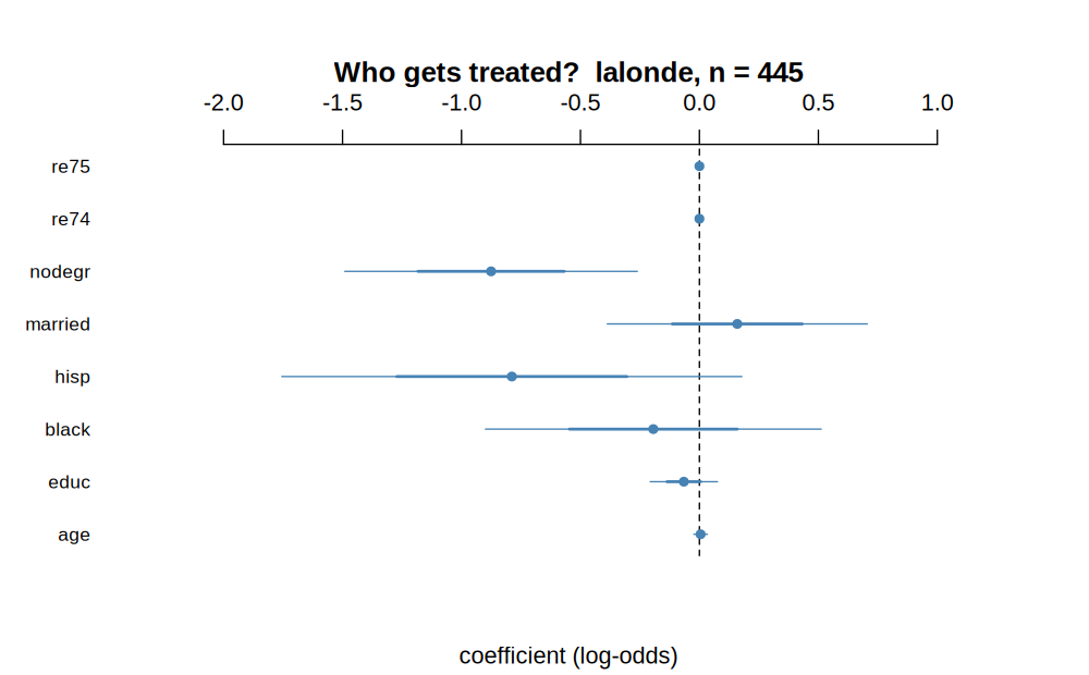
head(coef(sims)) # 1000 x 9 matrix of coefficient drawscoefplot() draws estimates with one- and
two-standard-error intervals — the default way to show a regression in
the book:
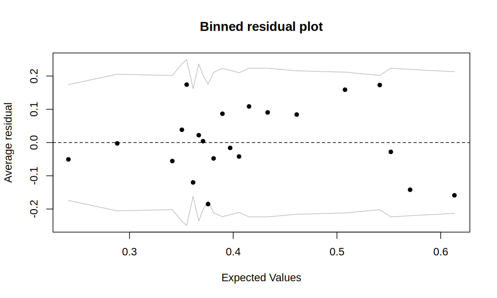
binnedplot() is the diagnostic for models with a
discrete response, where a scatterplot of residuals against fitted
values is useless because everything lands in two rows:
Also here: corrplot(),
discrete.histogram(), residual.plot(),
multicomp.plot(), triangleplot(),
traceplot().
matching()
and balance() — propensity score matchingmatching() does nearest-neighbour matching on a
propensity score; balance() summarises how well the matched
samples line up. The package ships lalonde, the dataset
Dehejia and Wahba (1999) used to evaluate these methods.
| Bayesian GLMs | bayesglm(), bayesglm.fit(),
bayespolr(), model.matrixBayes(),
contr.bayes.ordered(),
contr.bayes.unordered() |
| Simulation | sim(), mcsamp(), mcplot(),
traceplot(), extractDIC() |
| Summaries | display(), se.coef(),
se.fixef(), se.ranef(),
sigma.hat(), binned.resids(),
fround(), pfround() |
| Plots | coefplot(), binnedplot(),
corrplot(), discrete.histogram(),
residual.plot(), multicomp.plot(),
triangleplot() |
| Standardising | standardize(), rescale() |
| Matching | matching(), balance() |
| Small helpers | invlogit(), logit(),
read.columns(), go() |
Each has a help page: ?display, ?coefplot,
?sim.
GPL (>= 2), as in every published release of the package.