rifreg:
Estimate Recentered Influence Function Regressions
rifreg:
Estimate Recentered Influence Function Regressions![]()
![]()
![]()
![]()
Recentered influence function (RIF) regressions estimate the effects of small location shifts in continuous explanatory variables on a distributional statistic (e.g., quantile, variance or Gini coefficient) of an outcome variable as proposed by Firpo, Fortin, and Lemieux (2009a). In the special case of quantiles, RIF regressions are ‘unconditional quantile regressions’ capturing the association between explanatory variables and quantiles of the marginal distribution of an outcome variable.
You can either install the CRAN version of rifreg
install.packages("rifreg")or the latest development version from GitHub:
devtools::install_github("samumei/rifreg")Firpo, Fortin, and Lemieux (2009a) propose RIF regressions to estimate unconditional partial effects (UPE), i.e., the effects of small locations shifts in a continuous explanatory variable \(X\) on a distributional statistic \(\nu=\nu(F_Y)\) of an outcome variable \(Y\).
An influence function, as concept from robust statistics, informs about the extent a statistic of an empirical marginal distribution changes due to increasing the probability mass at value \(y\) by a small amount. A recentered influence functions is defined as the influence function recentered around the original distributional statistic: \[\text{RIF}(y;\nu,F_Y)= \nu(F_Y)+ \text{IF}(y;\nu,F_Y)\]
The expected value of a recentered influence function equals the original distributional statistic. Firpo et al. apply the law of iterated expectations to reformulate the distributional statistic in terms of the conditional expectations of the explanatory variables: \[\nu(F_Y) = \int \text{RIF}(y;\nu,F_Y) dF_Y= \int E(\text{RIF}(Y;\nu,F_Y)|X=x) dF_X(x)\]
This allows them to express the unconditional partial effects as average derivatives \[\alpha(\nu) = \int \frac{d E(\text{RIF}(Y;\nu,F_Y)|X=x)}{dx} dF_X(x).\]
Firpo et al. propose to approximate the conditional expectation of the RIF given the explanatory variables with a linear regression. The regression coefficients are consistent estimates of the average derivatives \(\widehat{\alpha}(\nu)\) if the conditional expectation of the RIF is linear and additive in \(X\) (see Firpo et al. 2009a, Rothe 2015: 328).
rifreg implements this approach. It first calculates the
RIF of the outcome variable \(Y\) and a
distributional statistic of interest \(\nu\). Then, it runs an OLS regression of
the transformed outcome variable \(Y\)
on the explanatory variables \(X\).
By default, the RIF of quantiles, the mean, the variance, the Gini
coefficient, the interquantile range and the quantile ratio are
available in rifreg. Moreover, the package allows to
calculate the RIF for additional statistics with user-written functions
(see example below). Cowell and
Flachaire (2007), Essama-Nssah
& Lambert (2012), and Rios-Avila (2020)
derive the influence functions for an array of distributional
statistics.
For the sake of illustration, consider the RIF of a quantile \(q_\tau = \inf_q \{q: F_Y(q) \geq \tau\}\). It is defined as \[\text{RIF}(y;q_\tau,F_Y) = q_\tau + \frac{\tau-1\{y \leq q_\tau\}}{f_Y(q_\tau)}, \] where \(1\{\}\) is the indicator function and \(f_Y(q_\tau)\) is the density at the quantile of interest. Thus, calculating the RIF requires estimating the sample quantile and the kernel density. The regression in the second step essentially amounts to a linear probability model (see Firpo et al., 2009a: 958, 961).
rifreg allows to bootstrap standard errors. Analytical
standard errors can be nontrivial when the RIF introduces an additional
estimation step. In particular, this is the case for quantiles where the
density has to be estimated (see Firpo,
Fortin, and Lemieux, 2009b).
Per default, summary.rifreg and
plot.rifregreturn heteroscedasticity-consistent standard
errors estimated with sandwich::sandwich() if the variance
is not bootstrapped. Note, however, that these standard errors do not
take the variance introduced by the RIF estimation step into
account.
In this basic example, we use a sample of the male wage data from the Current Population Survey from 1983 to 1985 as used in Firpo et al. (2009a).
library(rifreg)
#> Loading required package: ggplot2
data("men8385")We are interested in the unconditional quantile partial effects
(UQPE) of union membership on log hourly wages. We therefore estimate
RIF regressions on union status and control for demographic
characteristics. The parameter statistic specifies
quantiles as our distributional statistic of interest, while
probs defines the probabilities of the quantiles.
ffl_model <- log(wage) ~ union + nonwhite + married + education + experience
fit_uqr <- rifreg(ffl_model,
  data = men8385,
  weights = weights,
  statistic = "quantiles",
  probs = 1:9 / 10
)
#> Warning in density.default(x = dep_var, weights = weights/sum(weights, na.rm =
#> TRUE), : Selecting bandwidth *not* using 'weights'

#> Warning in density.default(x = dep_var, weights = weights/sum(weights, na.rm =
#> TRUE), : Selecting bandwidth *not* using 'weights'

#> Warning in density.default(x = dep_var, weights = weights/sum(weights, na.rm =
#> TRUE), : Selecting bandwidth *not* using 'weights'

#> Warning in density.default(x = dep_var, weights = weights/sum(weights, na.rm =
#> TRUE), : Selecting bandwidth *not* using 'weights'

#> Warning in density.default(x = dep_var, weights = weights/sum(weights, na.rm =
#> TRUE), : Selecting bandwidth *not* using 'weights'

#> Warning in density.default(x = dep_var, weights = weights/sum(weights, na.rm =
#> TRUE), : Selecting bandwidth *not* using 'weights'

#> Warning in density.default(x = dep_var, weights = weights/sum(weights, na.rm =
#> TRUE), : Selecting bandwidth *not* using 'weights'

#> Warning in density.default(x = dep_var, weights = weights/sum(weights, na.rm =
#> TRUE), : Selecting bandwidth *not* using 'weights'

#> Warning in density.default(x = dep_var, weights = weights/sum(weights, na.rm =
#> TRUE), : Selecting bandwidth *not* using 'weights'
fit_uqr
#> Rifreg coefficients:
#>                        rif_quantile_0.1 rif_quantile_0.2 rif_quantile_0.3
#> (Intercept)                0.9677792610      1.172213535      1.325780438
#> unionyes                   0.1895711045      0.295708058      0.387279233
#> nonwhiteyes               -0.1302511708     -0.184938936     -0.222993675
#> marriedyes                 0.2026240066      0.245443996      0.279350762
#> educationElementary       -0.3538349864     -0.477813514     -0.567215062
#> educationHS dropout       -0.3439659659     -0.330587413     -0.298250126
#> educationSome College      0.0548174446      0.115735854      0.159809840
#> educationCollege           0.1947681874      0.337966305      0.460910464
#> educationPost-graduate     0.1379931672      0.293259904      0.418461668
#> experience0-4             -0.5594535441     -0.693356537     -0.745007226
#> experience5-9             -0.0884216366     -0.165305983     -0.220432343
#> experience10-14           -0.0342842679     -0.074728354     -0.105916205
#> experience15-19           -0.0196581519     -0.025196360     -0.012289163
#> experience25-29           -0.0001536202      0.011879493      0.022959778
#> experience30-34           -0.0078147850     -0.015604532      0.005169821
#> experience35-39           -0.0122061390      0.008904716      0.037273681
#> experience>=40             0.0668346684      0.079740838      0.059595518
#>                        rif_quantile_0.4 rif_quantile_0.5 rif_quantile_0.6
#> (Intercept)                 1.547879317       1.73140047       1.88762362
#> unionyes                    0.376178021       0.32656124       0.21618201
#> nonwhiteyes                -0.211524098      -0.20089992      -0.15081897
#> marriedyes                  0.218579264       0.17922604       0.12516285
#> educationElementary        -0.527971072      -0.52330591      -0.39214911
#> educationHS dropout        -0.233202999      -0.21714277      -0.14751977
#> educationSome College       0.188642574       0.18926091       0.16383750
#> educationCollege            0.474357160       0.49065030       0.42622108
#> educationPost-graduate      0.476018944       0.52000299       0.48451657
#> experience0-4              -0.693878756      -0.63307290      -0.46205315
#> experience5-9              -0.291032518      -0.32426725      -0.27624894
#> experience10-14            -0.150302627      -0.18548369      -0.16165480
#> experience15-19            -0.063367268      -0.05039387      -0.03136320
#> experience25-29             0.011729605       0.04157812       0.05332638
#> experience30-34             0.003230684       0.03808255       0.04933966
#> experience35-39             0.023439785       0.03960192       0.05042873
#> experience>=40              0.020878466       0.02103064       0.03816951
#>                        rif_quantile_0.7 rif_quantile_0.8 rif_quantile_0.9
#> (Intercept)                  2.06188618      2.227099388     2.5134402077
#> unionyes                     0.11856052     -0.002668701    -0.1845993753
#> nonwhiteyes                 -0.11452478     -0.111328873    -0.1179041562
#> marriedyes                   0.10121558      0.080787039     0.0638341029
#> educationElementary         -0.31280611     -0.239681227    -0.2631182933
#> educationHS dropout         -0.12298166     -0.095285104    -0.0810231642
#> educationSome College        0.16102176      0.148442066     0.1717646078
#> educationCollege             0.44309979      0.452333786     0.6361150750
#> educationPost-graduate       0.53248414      0.608167593     0.8634031947
#> experience0-4               -0.41478063     -0.374038464    -0.4707231875
#> experience5-9               -0.29282199     -0.293692808    -0.3803066361
#> experience10-14             -0.19552918     -0.195891076    -0.2567293916
#> experience15-19             -0.05541812     -0.068011449    -0.1172958311
#> experience25-29              0.03431078      0.037563573     0.0765214464
#> experience30-34              0.06282862      0.079719979     0.0951429489
#> experience35-39              0.04234117      0.024843423     0.0710476353
#> experience>=40              -0.01446069     -0.023883275    -0.0002511195
The summary method returns the estimated coefficients
and the standard errors. Per default, summary returns
heteroscedasticity-consistent standard errors estimated if the variance
is not bootstrapped.
summary(fit_uqr)rifreg comes with a convenient plot function. It
illustrates the estimated UQPE across the distribution. The confidence
bands are based on the same standard errors as returned by
summary.
plot(fit_uqr, varselect = "unionyes")
#> Warning in plot.rifreg(fit_uqr, varselect = "unionyes"): Standard errors have not been bootstrapped!
#> Analytical s.e. do not take variance introduced by
#> estimating the RIF into account.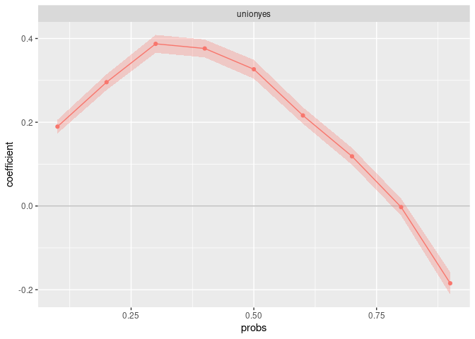
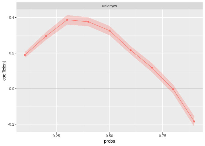
Setting bootstrap=TRUE bootstraps standard errors by
resampling from all observations and reestimating both the RIF and the
regression in every iteration. We can set the number of
bootstrap_iterations and the number of
cores.
fit_uqr <- rifreg(ffl_model,
  data = men8385,
  weights = weights,
  statistic = "quantiles",
  bootstrap = TRUE,
  bootstrap_iterations = 100,
  cores = 4,
  probs = 1:9 / 10
)
#> Warning in density.default(x = dep_var, weights = weights/sum(weights, na.rm =
#> TRUE), : Selecting bandwidth *not* using 'weights'

#> Warning in density.default(x = dep_var, weights = weights/sum(weights, na.rm =
#> TRUE), : Selecting bandwidth *not* using 'weights'

#> Warning in density.default(x = dep_var, weights = weights/sum(weights, na.rm =
#> TRUE), : Selecting bandwidth *not* using 'weights'

#> Warning in density.default(x = dep_var, weights = weights/sum(weights, na.rm =
#> TRUE), : Selecting bandwidth *not* using 'weights'

#> Warning in density.default(x = dep_var, weights = weights/sum(weights, na.rm =
#> TRUE), : Selecting bandwidth *not* using 'weights'

#> Warning in density.default(x = dep_var, weights = weights/sum(weights, na.rm =
#> TRUE), : Selecting bandwidth *not* using 'weights'

#> Warning in density.default(x = dep_var, weights = weights/sum(weights, na.rm =
#> TRUE), : Selecting bandwidth *not* using 'weights'

#> Warning in density.default(x = dep_var, weights = weights/sum(weights, na.rm =
#> TRUE), : Selecting bandwidth *not* using 'weights'

#> Warning in density.default(x = dep_var, weights = weights/sum(weights, na.rm =
#> TRUE), : Selecting bandwidth *not* using 'weights'
#> Bootstrapping Standard Errors...

plot(fit_uqr,
  varselect = "unionyes",
  confidence_interval = 0.95
)
rifreg performs RIF regressions for other distributional
statistics than quantiles. Per default, the “mean”, “variance”,
“quantiles”, “gini”, “interquantile_range” and “interquantile_ratio” are
available.
ffl_model2 <- wage ~ union + nonwhite + married + education + experience
fit_gini <- rifreg(ffl_model2,
  data = men8385,
  weights = weights,
  statistic = "gini"
)
fit_d9d1 <- rifreg(ffl_model2,
  data = men8385,
  weights = weights,
  statistic = "interquantile_ratio",
  probs = c(0.9, 0.1)
)
#> Warning in density.default(x = dep_var, weights = weights/sum(weights, na.rm =
#> TRUE), : Selecting bandwidth *not* using 'weights'
cbind(fit_gini$estimates, fit_d9d1$estimates)
#>                             rif_gini rif_iq_ratio_0.9_0.1
#> (Intercept)             3.421206e-01           4.94181575
#> unionyes               -1.018427e-01          -3.32876900
#> nonwhiteyes             1.584179e-02           1.18306521
#> marriedyes             -4.032892e-02          -2.38355788
#> educationElementary     4.962951e-02           3.47135861
#> educationHS dropout     4.645365e-02           4.15915721
#> educationSome College   7.404217e-03           0.05495204
#> educationCollege        5.411113e-02           0.27436327
#> educationPost-graduate  1.177852e-01           2.04326109
#> experience0-4           4.309944e-02           5.25521727
#> experience5-9          -3.926436e-02          -0.50972382
#> experience10-14        -4.094298e-02          -0.69812905
#> experience15-19        -1.736913e-02          -0.25813685
#> experience25-29         1.517589e-02           0.36083915
#> experience30-34         1.488841e-02           0.54174386
#> experience35-39         5.190609e-03           0.50875385
#> experience>=40 8.894634e-05 -0.88388009Users may write their own RIF function. Custom RIF functions must
specify a dep_var parameter for the outcome variable \(Y\), a weights for potential
sample weights, and probs. If they are not needed, they
must be set to NULL in the function definition
(e.g. probs = NULL).
The following example shows how to write the RIF for the top 10 percent income share and, then, to estimate the RIF regression using this custom function. The formula for this specific RIF can be found in Essam-Nssah & Lambert (2012) or Rios-Avila (2020).
ffl_model2 <- wage ~ union + nonwhite + married + education + experience

# custom RIF function for top 10% percent income share
custom_top_inc_share <- function(dep_var,
                                 weights,
                                 probs = NULL,
                                 top_share = 0.1) {
  top_share <- 1 - top_share
  weighted_mean <- weighted.mean(
    x = dep_var,
    w = weights
  )
  weighted_quantile <- Hmisc::wtd.quantile(
    x = dep_var,
    weights = weights,
    probs = top_share
  )
  lorenz_ordinate <- sum(dep_var[which(dep_var <= weighted_quantile)] *
    weights[which(dep_var <= weighted_quantile)]) /
    sum(dep_var * weights)
  if_lorenz_ordinate <- -(dep_var / weighted_mean) * lorenz_ordinate +
    ifelse(dep_var < weighted_quantile,
      dep_var - (1 - top_share) * weighted_quantile,
      top_share * weighted_quantile
    ) / weighted_mean
  rif_top_income_share <- (1 - lorenz_ordinate) - if_lorenz_ordinate
  rif <- data.frame(rif_top_income_share, weights)
  names(rif) <- c("rif_top_income_share", "weights")
  return(rif)
}

fit_top_10 <- rifreg(ffl_model2,
  data = men8385,
  weights = weights,
  statistic = "custom",
  custom_rif_function = custom_top_inc_share,
  top_share = 0.1
)

fit_top_10
#> Rifreg coefficients:
#>                        rif_top_income_share
#> (Intercept)                    0.2603167792
#> unionyes                      -0.0683100301
#> nonwhiteyes                    0.0089816022
#> marriedyes                    -0.0219216751
#> educationElementary            0.0252425640
#> educationHS dropout            0.0221077827
#> educationSome College          0.0025577576
#> educationCollege               0.0386916446
#> educationPost-graduate         0.0804506915
#> experience0-4                  0.0110458948
#> experience5-9                 -0.0227483071
#> experience10-14               -0.0286122339
#> experience15-19               -0.0115646111
#> experience25-29                0.0114751845
#> experience30-34                0.0041189370
#> experience35-39                0.0009313563
#> experience>=40 0.0111984967To validate the functions and provide users with an additional example, we replicate the RIF regression estimates in Firpo et al. (2009a: 962-966). In their empirical example, Firpo et al. estimate the impact of union status on log wages using a large sample of 266’956 male U.S. workers from 1983-1985 based on the Outgoing Rotation Group (ORG) supplement of the Current Population Survey. To reproduce the code below, make sure you download the entire data set from the journal’s website.
library("dplyr")
#>
#> Attaching package: 'dplyr'
#> The following objects are masked from 'package:stats':
#>
#>     filter, lag
#> The following objects are masked from 'package:base':
#>
#>     intersect, setdiff, setequal, union

## getting the data from the journal's website
# url <- "https://www.econometricsociety.org/publications/econometrica/2009/05/01/unconditional-quantile-regressions/supp/6822_data%20and%20programs_0.zip"
# download.file(url = url, destfile = "6822_data%20and%20programs_0.zip")
# men8385 <- readstata13::read.dta13(file = unzip("6822_data%20and%20programs_0.zip","men8385.dta"))

## Load data
men8385 <- readstata13::read.dta13("data-raw/men8385.dta")

# Save dummies as factor variables
# nine potential experience categories (each of five years gap)
men8385$experience <- 5
men8385[which(men8385$ex1 == 1), "experience"] <- 1
men8385[which(men8385$ex2 == 1), "experience"] <- 2
men8385[which(men8385$ex3 == 1), "experience"] <- 3
men8385[which(men8385$ex4 == 1), "experience"] <- 4
# 5 = reference group
men8385[which(men8385$ex6 == 1), "experience"] <- 6
men8385[which(men8385$ex7 == 1), "experience"] <- 7
men8385[which(men8385$ex8 == 1), "experience"] <- 8
men8385[which(men8385$ex9 == 1), "experience"] <- 9

# Education
men8385$education <- 2
men8385[which(men8385$ed0 == 1), "education"] <- 0
men8385[which(men8385$ed1 == 1), "education"] <- 1
# high school = reference group
men8385[which(men8385$ed3 == 1), "education"] <- 3
men8385[which(men8385$ed4 == 1), "education"] <- 4
men8385[which(men8385$ed5 == 1), "education"] <- 5

men8385$education <- as.character(men8385$education)
men8385$experience <- as.character(men8385$experience)
men8385$experience <- dplyr::recode_factor(men8385$experience,
  "5" = "20-24",
  "1" = "0-4",
  "2" = "5-9",
  "3" = "10-14",
  "4" = "15-19",
  "6" = "25-29",
  "7" = "30-34",
  "8" = "35-39",
  "9" = ">=40"
)

men8385$education <- dplyr::recode_factor(men8385$education,
  "2" = "High School",
  "0" = "Elementary",
  "1" = "HS dropout",
  "3" = "Some College",
  "4" = "College",
  "5" = "Post-graduate"
)

# Save log wage as wage hourly wage in dollars
men8385$wage <- exp(men8385$lwage)

# Rename/relevel remaining indicators
men8385$union <- as.factor(men8385$covered)
men8385$covered <- NULL

men8385$married <- as.factor(men8385$marr)
men8385$marr <- NULL
men8385$nonwhite <- as.factor(men8385$nonwhite)
levels(men8385$married) <- levels(men8385$nonwhite) <- levels(men8385$union) <- c("no", "yes")

# Rename weight and education in years variable
names(men8385)[names(men8385) == "eweight"] <- "weights"
names(men8385)[names(men8385) == "educ"] <- "education_in_years"
names(men8385)[names(men8385) == "exper"] <- "experience_in_years"

# Check experience and age groups
men8385 %>%
  group_by(experience) %>%
  dplyr::summarise(
    min = min(experience_in_years, na.rm = TRUE),
    max = max(experience_in_years, na.rm = TRUE)
  )
#> # A tibble: 9 × 3
#>   experience   min   max
#>   <fct>      <dbl> <dbl>
#> 1 20-24         20    24
#> 2 0-4            0     4
#> 3 5-9            5     9
#> 4 10-14         10    14
#> 5 15-19         15    19
#> 6 25-29         25    29
#> 7 30-34         30    34
#> 8 35-39         35    39
#> 9 >=40          40    58

men8385 %>%
  group_by(education) %>%
  dplyr::summarise(
    min = min(education_in_years, na.rm = TRUE),
    max = max(education_in_years, na.rm = TRUE)
  )
#> # A tibble: 6 × 3
#>   education       min   max
#>   <fct>         <dbl> <dbl>
#> 1 High School      12    12
#> 2 Elementary        0     8
#> 3 HS dropout        9    11
#> 4 Some College     13    15
#> 5 College          16    16
#> 6 Post-graduate    17    18

# Select relevant variables
sel_vars <- c("wage", "union", "nonwhite", "married",
              "education", "experience", "weights",
              "age", "education_in_years", "experience_in_years")
men8385 <- men8385[, sel_vars]The model is specified as in Firpo, Fortin, and Lemieux (2007a), omitting weights, computing bootstrapped standard errors with 200 iterations and setting a fixed bandwidth of 0.06 for the kernel density estimation. We also compute a OLS model for comparison with the original results.
library(rifreg)

set.seed(121095)
ffl_model_2009 <- log(wage) ~ union + nonwhite + married + education + experience
ffl_uqr_fit <- rifreg(
  formula = ffl_model_2009,
  data = men8385,
  statistic = "quantiles",
  probs = seq(0.05, 0.95, 0.05),
  bw = 0.06,
  bootstrap = TRUE,
  bootstrap_iterations = 200,
  cores = 1
)
#> Bootstrapping Standard Errors...

ffl_ols_fit <- lm(
  formula = ffl_model_2009,
  data = men8385
)estimates <- data.frame(
ffl_uqr_fit$estimates[1:9,
c("rif_quantile_0.1",
"rif_quantile_0.5",
"rif_quantile_0.9")])
standard_errors <- data.frame(
ffl_uqr_fit$bootstrap_se[1:9,
c("rif_quantile_0.1",
"rif_quantile_0.5",
"rif_quantile_0.9")])
results <- cbind(estimates, standard_errors)[, c(1, 4, 2, 5, 3, 6)]
results$ols <- ffl_ols_fit$coefficients[1:9]
names(results) <- c("Coefficient 0.1", "SE",
"Coefficient 0.5", "SE",
"Coefficient 0.9", "SE",
"OLS")
knitr::kable(results, digits = 3)| Coefficient 0.1 | SE | Coefficient 0.5 | SE | Coefficient 0.9 | SE | OLS | |
|---|---|---|---|---|---|---|---|
| (Intercept) | 0.970 | 0.005 | 1.735 | 0.006 | 2.511 | 0.009 | 1.742 |
| unionyes | 0.195 | 0.003 | 0.336 | 0.004 | -0.135 | 0.004 | 0.179 |
| nonwhiteyes | -0.116 | 0.005 | -0.164 | 0.004 | -0.099 | 0.004 | -0.134 |
| marriedyes | 0.194 | 0.004 | 0.156 | 0.003 | 0.043 | 0.004 | 0.140 |
| educationElementary | -0.306 | 0.008 | -0.451 | 0.006 | -0.240 | 0.005 | -0.351 |
| educationHS dropout | -0.344 | 0.006 | -0.194 | 0.004 | -0.068 | 0.003 | -0.190 |
| educationSome College | 0.058 | 0.004 | 0.178 | 0.004 | 0.153 | 0.005 | 0.133 |
| educationCollege | 0.196 | 0.004 | 0.464 | 0.005 | 0.581 | 0.008 | 0.406 |
| educationPost-graduate | 0.138 | 0.004 | 0.522 | 0.006 | 0.843 | 0.012 | 0.478 |
Our results largely match those by Firpo, Fortin, and Lemieux (2009a: 964, Table I). The OLS results are identical as expected. The RIF regression results differ only in a few instances at the third decimal place from the original paper.
rifreg_plot <- plot(ffl_uqr_fit, varselect = "unionyes")rifreg_plot +
geom_hline(yintercept = ffl_ols_fit$coefficients["unionyes"],
linetype = "dashed") +
geom_text(aes(x = 0.8,
y = ffl_ols_fit$coefficients["unionyes"] + 0.03,
label = "OLS estimate"),
color = "black") +
ylab("Effect of Union") +
xlab("Quantiles") +
labs(title = "Unconditional Quantile Regression in R") +
theme(strip.background = element_blank(),
strip.text.x = element_blank())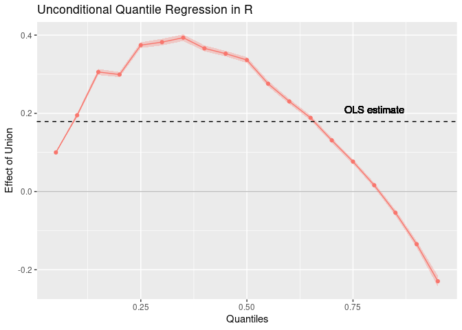
Looking at the plots, we see that our plots correspond to those
presented by Firpo, Fortin, and Lemieux (2009a: 965). The plot example
illustrates, how the plot from the generic rifreg::plot()
function can be further enhanced, for instance with a horizontal line
indicating the OLS coefficient for comparison.
This validation example illustrates that the rifreg
package works as intended in computing RIF regressions and reliably
yields the expected results.
David Gallusser & Samuel Meier
Cowell, Frank A., and Emmanuel Flachaire. 2007. “Income distribution and inequality measurement: The problem of extreme values.” Journal of Econometrics 141: 1044–1072.
Essama-Nssah, Boniface, and Peter J. Lambert. 2012. “Influence Functions for Policy Impact Analysis.” In John A. Bishop and Rafael Salas, eds., Inequality, Mobility and Segregation: Essays in Honor of Jacques Silber. Bigley, UK: Emerald Group Publishing Limited.
Firpo, Sergio, Nicole M. Fortin, and Thomas Lemieux. 2007a. “Unconditional Quantile Regressions.” Tech- nical Working Paper 339, National Bureau of Economic Research. Cambridge, MA.
Firpo, Sergio, Nicole M. Fortin, and Thomas Lemieux. 2009a. “Unconditional Quantile Regressions.” Econometrica 77(3): 953-973.
Firpo, Sergio, Nicole M. Fortin, and Thomas Lemieux. 2009b. “Supplement to ‘Unconditional Quantile Regressions’.” Econometrica Supplemental Material, 77.
Rios-Avila, Fernando. 2020. “Recentered influence functions (RIFs) in Stata: RIF regression and RIF decomposition.” The Stata Journal 20(1): 51-94.
Rothe, Christoph. 2015. “Decomposing the Composition Effect. The Role of Covariates in Determining Between-Group Differences in Economic Outcomes.” Journal of Business & Economic Statistics 33(3): 323-337.