splitGraph: Dataset Dependency Graphs for Leakage-Aware Evaluation

splitGraph is an R package for representing biomedical dataset structure as a typed dependency graph so that leakage-relevant relationships can be made explicit, validated, queried, and converted into deterministic split constraints.

It does not fit models, run preprocessing pipelines, or generate resamples by itself. Its job is to encode dataset structure before evaluation so that overlap, provenance, and time-ordering assumptions are inspectable instead of implicit.

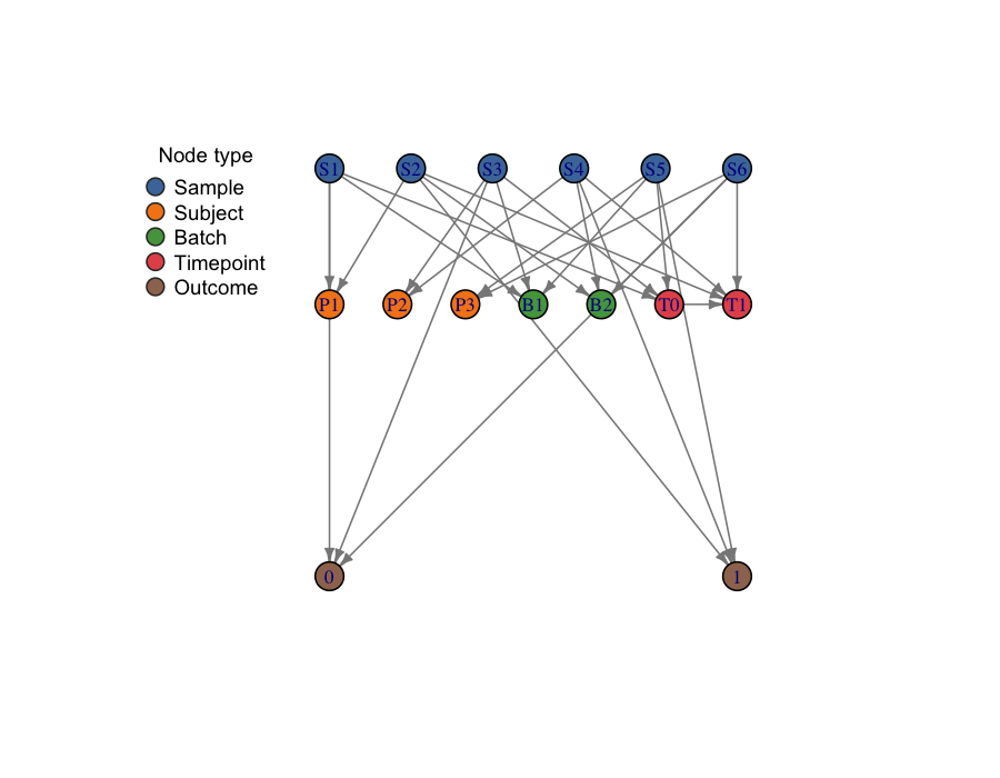
The plot above shows six samples (blue) that share three subjects (orange), two batches (green), two timepoints (red), and two outcome classes (brown). A plain vfold_cv on this dataset would violate subject, batch, and time structure at the same time — and that is exactly what the graph is designed to make visible.

Why It Exists

In biomedical evaluation workflows, leakage often comes from dataset structure rather than obvious coding mistakes. Samples may share:

the same subject
the same batch
the same study
the same collection timepoint
the same assay provenance
the same derived feature set
the same outcome definition

If those relationships are not modeled explicitly, a train/test split can look correct while still violating the intended scientific separation.

splitGraph makes those dependencies first-class objects.

What It Does (and Does Not Do)

Does:

metadata ingestion with canonical ID normalization
one-shot graph construction from canonical metadata via graph_from_metadata()
typed node and edge constructors backed by igraph
structural, semantic, and leakage-relevant validation
typed query and traversal helpers
projected sample-dependency detection
split-constraint derivation for subject, batch, study, time, and composite modes
translation of constraints into a stable, tool-agnostic split_spec
split-spec preflight validation and leakage summary helpers
typed layered plot() method with per-type colors and a node-type legend
print(), summary(), and as.data.frame() on all core S3 objects

Does not:

fit models or run preprocessing pipelines
generate resamples (rsample does that)
implement leakage-aware training workflows or fit models
provide a general-purpose graph analytics toolkit

The package is intentionally narrow: dataset dependency structure for leakage-aware evaluation design.

Installation

Development version from GitHub:

install.packages("remotes")
remotes::install_github("selcukorkmaz/splitGraph")

Quick Start

The fastest path is graph_from_metadata(), which auto-detects canonical columns in a metadata frame and assembles a validated dependency_graph:

library(splitGraph)

meta <- data.frame(
  sample_id    = c("S1", "S2", "S3", "S4", "S5", "S6"),
  subject_id   = c("P1", "P1", "P2", "P2", "P3", "P3"),
  batch_id     = c("B1", "B2", "B1", "B2", "B1", "B2"),
  timepoint_id = c("T0", "T1", "T0", "T1", "T0", "T1"),
  time_index   = c(0, 1, 0, 1, 0, 1),
  outcome_value = c(0, 1, 0, 1, 1, 0)
)

g <- graph_from_metadata(meta, graph_name = "demo")
plot(g)

validation <- validate_graph(g)
subject_constraint <- derive_split_constraints(g, mode = "subject")
split_spec <- as_split_spec(subject_constraint, graph = g)
validate_split_spec(split_spec)
summarize_leakage_risks(g, constraint = subject_constraint, split_spec = split_spec)

For full control over node labels, attribute columns, and non-canonical relations, use create_nodes() / create_edges() / build_dependency_graph() directly.

Downstream Handoff

split_spec is the tool-agnostic handoff object produced by as_split_spec(). splitGraph does not know about any particular resampling package — downstream consumers are expected to provide their own adapters so that splitGraph stays neutral and has no runtime dependency on them.

The typical end-to-end flow is:

graph_from_metadata(meta) → typed dependency_graph
derive_split_constraints(g, mode = ...) → split_constraint
as_split_spec(constraint, graph = g) → split_spec
adapter in the downstream package → native resamples

The sample_data frame carried by split_spec exposes exactly what an adapter needs: sample_id for joining against the observation frame, group_id for grouped resampling, batch_group / study_group for blocking, and order_rank for ordered evaluation. An adapter can be built on top of, for example, rsample::group_vfold_cv() (grouped CV keyed to group_id) or rsample::rolling_origin() (ordered evaluation keyed to order_rank).

Core Concepts

Node types

Sample, Subject, Batch, Study, Timepoint, Assay, FeatureSet, Outcome

Canonical edge types

sample_belongs_to_subject
sample_processed_in_batch
sample_from_study
sample_collected_at_timepoint
sample_measured_by_assay
sample_uses_featureset
sample_has_outcome
subject_has_outcome
timepoint_precedes
featureset_generated_from_study
featureset_generated_from_batch

Main S3 objects

graph_node_set, graph_edge_set, dependency_graph, depgraph_validation_report, graph_query_result, split_constraint, split_spec, split_spec_validation, leakage_risk_summary.

Main Functions

Layer	Functions
Ingestion and construction	`ingest_metadata()`, `graph_from_metadata()`, `create_nodes()`, `create_edges()`, `build_dependency_graph()`, `dependency_graph()`, `as_igraph()`
Validation	`validate_graph()`, `validate_split_spec()`
Queries	`query_node_type()`, `query_edge_type()`, `query_neighbors()`, `query_paths()`, `query_shortest_paths()`, `detect_dependency_components()`, `detect_shared_dependencies()`
Constraint derivation	`derive_split_constraints()`, `grouping_vector()`
Split-spec translation	`as_split_spec()`, `summarize_leakage_risks()`

Example Queries

query_node_type(g, "Subject")
query_edge_type(g, "sample_processed_in_batch")
query_neighbors(g, node_ids = "sample:S1", edge_types = "sample_belongs_to_subject")
detect_shared_dependencies(g, via = "Batch")
detect_dependency_components(g, via = c("Subject", "Batch"))

Example Split Designs

subject_constraint <- derive_split_constraints(g, mode = "subject")
batch_constraint   <- derive_split_constraints(g, mode = "batch")
study_constraint   <- derive_split_constraints(g, mode = "study")
time_constraint    <- derive_split_constraints(g, mode = "time")

strict_composite <- derive_split_constraints(
  g, mode = "composite", strategy = "strict",
  via = c("Subject", "Batch")
)

rule_based_composite <- derive_split_constraints(
  g, mode = "composite", strategy = "rule_based",
  priority = c("batch", "study", "subject", "time")
)

Plot Method

plot(g) renders a typed, layered layout with per-type node colors and an auto-generated node-type legend. Layers: Sample (top), peer dependencies (Subject / Batch / Study / Timepoint) in the middle band, Assay / FeatureSet next, Outcome (bottom).

plot(g)                              # typed layered layout (default)
plot(g, layout = "sugiyama")         # alternative hierarchical layout
plot(g, show_labels = FALSE)         # hide node labels on dense graphs
plot(g, legend = FALSE)              # suppress the legend
plot(g, legend_position = "bottomright")
plot(g, node_colors = c(Sample = "#000000"))  # override type colors

Citation

citation("splitGraph")

produces:

Korkmaz S (2026). splitGraph: Dataset Dependency Graphs for Leakage-Aware Evaluation. R package version 0.1.0. https://github.com/selcukorkmaz/splitGraph

License

MIT. See LICENSE.

Appendix: Design Guarantees

The package prefers explicit failure over silent guessing. In particular:

unknown sample IDs, ambiguous direct assignments, and conflicting duplicate nodes or edges are rejected rather than silently resolved
contradictory time-order metadata are rejected rather than reconciled arbitrarily
validation truth is not changed by severity filters, and generated split specs are re-validated against the package’s own preflight rules