
Vignettes
Guides
Case studies
transitiontrees models how categorical processes unfold:
how one state follows another in weekly engagement, collaborative
regulation or the turns of a human-AI conversation. It fits
variable-order transition trees, also known as prediction suffix trees
(Ron, Singer, & Tishby, 1996) or variable-length Markov chains
(Bühlmann & Wyner, 1999), in which the length of history used to
predict the next state differs from one history to another: the tree is
deep where earlier states change the prediction and shallow where they
do not. Each branch is a pathway, a run of recent states with the
distribution of the state that followed it. The package reports which
pathways occur, which change the prediction relative to a shorter
history, how stable they are under the bootstrap, and whether they
differ between groups, separating differences in what follows a history
from differences in how often the history occurs.
Trees are fitted from wide sequence data, long event logs and sequence-bearing network objects; pruned by likelihood-ratio tests or information criteria; evaluated by log likelihood, information criteria and perplexity; and used to predict, score, simulate and impute sequences. Results are tidy data frames, and plots are ggplot2 objects.
For a sequence \(x_1, \dots, x_T\)
over a set of states \(S\), a context
is a run of recent states \(c = (x_{t-k},
\dots, x_{t-1})\), and each context in the tree carries a
next-state distribution \(P(x_t = s \mid
c)\). A new state is predicted from the longest suffix of its
history that is a context in the tree, \(c^*(t)\), so that \(\hat P(x_t \mid x_1, \dots, x_{t-1}) = \hat P(x_t
\mid c^*(t))\). A context receives a node when it is no longer
than max_depth and occurs at least min_count
times; its distribution is estimated from the counts \(N(c, s)\) and smoothed so that unobserved
next states keep a small probability. A leaf \(c\) is pruned when its counts are
consistent with the prediction of its parent \(\pi(c)\), the context with the oldest state
removed, under the likelihood-ratio test
\[ G^2(c) = 2 \sum_{s} N(c, s) \log \frac{N(c, s)}{N(c)\, \tilde p(s \mid \pi(c))} \;\le\; \chi^2_{|S| - 1,\, 1 - \alpha}, \]
or under an AIC or BIC penalty (Ron, Singer, & Tishby, 1996;
Bühlmann & Wyner, 1999; Gabadinho & Ritschard, 2016). Pathways
are written oldest state first (Average -> Disengaged),
and the empty context is shown as (start).
install.packages("transitiontrees")

# development version
install.packages("remotes")
remotes::install_github("mohsaqr/transitiontrees")engagement holds the weekly engagement states
(Active, Average, Disengaged) of
1,000 students. The tree below allows histories of up to three weeks,
and pruning keeps the contexts that pass the \(G^2\) test.
library(transitiontrees)

tree <- context_tree(engagement, max_depth = 3, min_count = 10)
pruned <- prune_tree(tree, criterion = "G2", alpha = 0.05)
model_fit(pruned)
#>   logLik df  nobs   AIC   BIC perplexity
#> 1 -16181 20 24555 32403 32565       1.93
Pathways that change the prediction made from the shorter history are
ranked by divergent_pathways().
divergent_pathways(pruned, top = 5)
#>                              pathway depth count likely_next next_probability divergence
#> 1                         Disengaged     1  6598  Disengaged            0.786     0.9453
#> 2                             Active     1 11894      Active            0.859     0.4183
#> 3                            Average     1  5063     Average            0.548     0.3836
#> 4     Active -> Disengaged -> Active     3    22      Active            0.727     0.2546
#> 5 Active -> Disengaged -> Disengaged     3   449  Disengaged            0.788     0.0113
#>   changes_prediction
#> 1               TRUE
#> 2              FALSE
#> 3               TRUE
#> 4              FALSE
#> 5              FALSE
plot() draws the tree from the root on the left, with
node size proportional to the context count and the modal next state
under each node.
plot(pruned)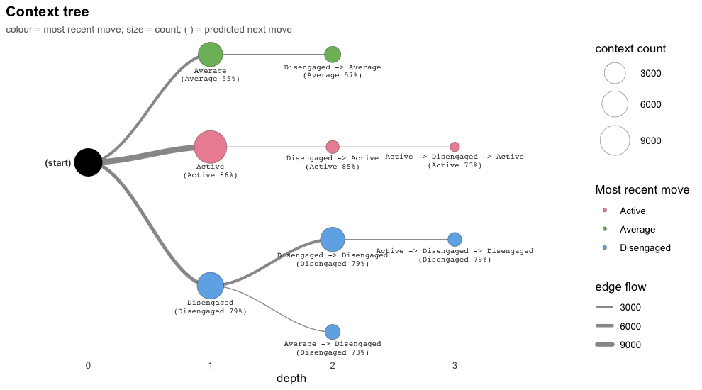
plot of chunk plot-tree
predict() applies the longest-suffix rule to new
histories; with tidy = TRUE it returns one row per history
with the context used and the next-state distribution.
predict(pruned, newdata = list(c("Active", "Average"),
                               c("Average", "Disengaged")),
        tidy = TRUE)
#>   id               history               context  predicted probability Active Average
#> 1  1     Active -> Average               Average    Average       0.548 0.3052   0.548
#> 2  2 Average -> Disengaged Average -> Disengaged Disengaged       0.734 0.0556   0.210
#>   Disengaged
#> 1      0.147
#> 2 0.734transitiontrees is written by Mohammed Saqr and Sonsoles López-Pernas. Mohammed Saqr
maintains the package. Questions and bug reports can be submitted
through the repository
issue tracker. The package citation is available through
citation("transitiontrees").
Bühlmann, P., & Wyner, A. J. (1999). Variable length Markov chains. The Annals of Statistics, 27(2), 480–513. https://doi.org/10.1214/aos/1018031204
Gabadinho, A., & Ritschard, G. (2016). Analyzing state sequences with probabilistic suffix trees: The PST R package. Journal of Statistical Software, 72(3). https://doi.org/10.18637/jss.v072.i03
Ron, D., Singer, Y., & Tishby, N. (1996). The power of amnesia: Learning probabilistic automata with variable memory length. Machine Learning, 25(2–3), 117–149. https://doi.org/10.1023/A:1026490906255